This post, and this post on the Chow ring, both serve the same purpose: to work out some explicit examples in intersection theory.
Unlike the above post on the Chow ring, however, some of the content of this post can be found in a previous post of mine on the Grothendieck ring of projective space. There are a number of small changes and corrections I’ve wanted to make since writing that post. Some of the changes I’ve incorporated between that post and this one are: small changes in notation which serve to clarify the properties of the two Grothendieck groups, adding some detail to the functorial behavior of the groups and discussing the ring structure, completing a proof on the generation of the Grothendieck group of projective space using the localization sequence.
In later posts, I’ll work out descriptions for the Grothendieck ring(s) of Grassmannians and Flag varieties. The main example of this post is projective space in section 1.
Caution: When I talk about varieties, I mean a separated scheme of finite type over a field. It will be blatantly clear the definitions and theorems included in this post extend to more general situations. Since this post is about examples, which all happen to be varieties, I don’t really care about the difference here…
Recollections from “K-theory and G-theory”
The purpose of this section is to summarize some of the various functorial properties of algebraic K-theory. We focus on the 0th higher K-group, much as the post on the Chow ring focuses on the 0th higher Chow group. References where this material is developed (without the use of homotopy theory) include the original source, [SGA6], and the master’s thesis of Javanpeykar, [Jav]. There is also a survey article by Levine, [Lev].
(0.1) Definition: let  be a variety. We define the group
  as the free abelian group on isomorphism classes of finite rank locally free sheaves on with the relations
 ![[\mathcal{F}]=[\mathcal{E}]+[\mathcal{G}]](https://s0.wp.com/latex.php?latex=%5B%5Cmathcal%7BF%7D%5D%3D%5B%5Cmathcal%7BE%7D%5D%2B%5B%5Cmathcal%7BG%7D%5D&bg=f7f3ee&fg=333333&s=0&c=20201002) whenever there is an exact sequence
whenever there is an exact sequence  . We define the group
  similarly, replacing everywhere locally free sheaves by coherent sheaves. We call these groups the K-theory and G-theory of respectively.
Remarks: if, in the definition above, we used infinite rank sheaves or quasi-coherent sheaves then the respective group would be 0. To see this, note  and
and ![[A\oplus B]=[A]+[B]](https://s0.wp.com/latex.php?latex=%5BA%5Coplus+B%5D%3D%5BA%5D%2B%5BB%5D&bg=f7f3ee&fg=333333&s=0&c=20201002) hence
hence ![[A]=0](https://s0.wp.com/latex.php?latex=%5BA%5D%3D0&bg=f7f3ee&fg=333333&s=0&c=20201002) .
.
Since the categories are equivalent, we could have used vector bundles instead of sheaves to define K-theory.
The class of a bounded complex of coherent sheaves makes sense in G-theory since, by splicing, we can show it is equivalent to the alternating sum of its homology sheaves. For the relations of G-theory, we could thus have instead used arbitrary length exact sequences and alternating sums in the definition. Note this doesn’t work for K-theory because the homology sheaves are usually not locally free.
We use nonstandard notation and terminology. Unlike most other sources, we treat the K-theory and G-theory groups as completely different objects. The reason this is nonstandard is because both the K-theory and G-theory defined above arise from a more general procedure and we have just applied this procedure to different categories.
We’ll start with some observations about K-theory.
(0.2) Lemma: for any variety , the group is a ring under the operation ![[\mathcal{F}]\cdot[\mathcal{E}]=[\mathcal{F}\otimes_{\mathcal{O}_X}\mathcal{E}]](https://s0.wp.com/latex.php?latex=%5B%5Cmathcal%7BF%7D%5D%5Ccdot%5B%5Cmathcal%7BE%7D%5D%3D%5B%5Cmathcal%7BF%7D%5Cotimes_%7B%5Cmathcal%7BO%7D_X%7D%5Cmathcal%7BE%7D%5D&bg=f7f3ee&fg=333333&s=0&c=20201002) . The multiplication this defines is associative, commutative, and bilinear. Given a morphism of varieties,
. The multiplication this defines is associative, commutative, and bilinear. Given a morphism of varieties,  , there is a morphism
  which is determined by its action on classes
 ![f^*([\mathcal{F}])=[f^*\mathcal{F}]](https://s0.wp.com/latex.php?latex=f%5E%2A%28%5B%5Cmathcal%7BF%7D%5D%29%3D%5Bf%5E%2A%5Cmathcal%7BF%7D%5D&bg=f7f3ee&fg=333333&s=0&c=20201002) . These morphisms make
. These morphisms make  into a contravariant functor from the category of varieties to the category of commutative rings. That is to say the map induced by the identity is the identity and the map induced by a composition is the composition of the induced maps.
Proof. The first result follows from the fact tensoring by a locally free is exact. The properties of the multiplication are inherited from those of the tensor product. That the definition for the pullback induces a well-defined map on K-theory follows from the fact the pullback of a short exact sequence of locally frees is a short exact sequence of locally frees (a locally free sheaf is acyclic for the higher Tor sheaves so from the long exact Tor sequence all terms >1 vanish). The functorality of  (on K-theory) is inherited from that of (on sheaves).
Surprisingly that’s all I want to say about K-theory, for now. The heart of this post is about intersection theoretic properties one can extract from these groups and, for this we’ll need to use G-theory.
(0.3) Lemma: for any variety , the group is a module over . The multiplication takes the class of a locally free sheaf in and the class of a coherent sheaf in to the class of their tensor product in .
Let be a morphism of varieties. If  is proper, there is a map
  defined by
 ![f_*([\mathcal{F}])=\sum_{i=0}^\infty (-1)^i [R^if_*(\mathcal{F})]](https://s0.wp.com/latex.php?latex=f_%2A%28%5B%5Cmathcal%7BF%7D%5D%29%3D%5Csum_%7Bi%3D0%7D%5E%5Cinfty+%28-1%29%5Ei+%5BR%5Eif_%2A%28%5Cmathcal%7BF%7D%29%5D&bg=f7f3ee&fg=333333&s=0&c=20201002) . These maps are covariantly functorial when defined.
. These maps are covariantly functorial when defined.
If is flat, there is a map  defined by . When has finite Tor-dimension, we can drop the assumption is flat; in this case we write
  and it is defined
 ![f^!([\mathcal{F}])=\sum_{i=0}^\infty (-1)^i [L^if^* \mathcal{F}]](https://s0.wp.com/latex.php?latex=f%5E%21%28%5B%5Cmathcal%7BF%7D%5D%29%3D%5Csum_%7Bi%3D0%7D%5E%5Cinfty+%28-1%29%5Ei+%5BL%5Eif%5E%2A+%5Cmathcal%7BF%7D%5D&bg=f7f3ee&fg=333333&s=0&c=20201002) . These are contravariantly functorial when defined.
. These are contravariantly functorial when defined.
There is also the projection formula:  for
for  and
and  .
.
Proof. These results, as in lemma (0.2), all derive from the corresponding results on sheaves. That the maps  are well-defined is a result of homological algebra: for proper morphisms the higher direct images are coherent, and vanish above the dimension of the largest fiber of the map ; for flat morphisms the pullback is exact on coherent sheaves and to drop the flatness assumption we impose finite Tor-dimension so the higher inverse images vanish in sufficiently large degrees; both direct image and inverse image take short exact sequences of sheaves to long exact sequences of higher-images, which, in turn, shows the above maps are well-defined. The projection formula follows from the same formula on sheaves.
Let’s now show the functorality of compositions of these morphisms on G-theory. Suppose then  are morphisms of varieties, with
  of finite Tor-dimension and suppose further
  have enough finite locally-frees (all coherent sheaves on either admit surjections from a finite locally free sheaf). We actually need both of these conditions since we only know the derived functor isomorphism
  in this setting. In this case there is a spectral sequence computing the right side starting from the left:
 .
.
For any bounded spectral sequence we have ![\sum_i(-1)^i[E_r^{p+ir,q-ir+i}]=\sum_i(-1)^i[E_{r+1}^{p+ir,q-ir+i}]](https://s0.wp.com/latex.php?latex=%5Csum_i%28-1%29%5Ei%5BE_r%5E%7Bp%2Bir%2Cq-ir%2Bi%7D%5D%3D%5Csum_i%28-1%29%5Ei%5BE_%7Br%2B1%7D%5E%7Bp%2Bir%2Cq-ir%2Bi%7D%5D&bg=f7f3ee&fg=333333&s=0&c=20201002) , since we can replace any complex — the terms on the left — by its homology sheaves — the terms on the right. Summing over all
, since we can replace any complex — the terms on the left — by its homology sheaves — the terms on the right. Summing over all  we find
 ![\sum_{p,q}(-1)^{p+q}[E_r^{p+q}]=\sum_{p,q} (-1)^{p+q}[E_{r+1}^{p+q}]](https://s0.wp.com/latex.php?latex=%5Csum_%7Bp%2Cq%7D%28-1%29%5E%7Bp%2Bq%7D%5BE_r%5E%7Bp%2Bq%7D%5D%3D%5Csum_%7Bp%2Cq%7D+%28-1%29%5E%7Bp%2Bq%7D%5BE_%7Br%2B1%7D%5E%7Bp%2Bq%7D%5D&bg=f7f3ee&fg=333333&s=0&c=20201002) . Applying this to the spectral sequence mentioned above (using finite Tor-dimension to imply boundedness) gives
. Applying this to the spectral sequence mentioned above (using finite Tor-dimension to imply boundedness) gives
![f^!\circ g^!([\mathcal{F}])=\sum_{p+q}(-1)^{p+q}[L^pf^*(L^qg^*(\mathcal{F}))]](https://s0.wp.com/latex.php?latex=f%5E%21%5Ccirc+g%5E%21%28%5B%5Cmathcal%7BF%7D%5D%29%3D%5Csum_%7Bp%2Bq%7D%28-1%29%5E%7Bp%2Bq%7D%5BL%5Epf%5E%2A%28L%5Eqg%5E%2A%28%5Cmathcal%7BF%7D%29%29%5D&bg=f7f3ee&fg=333333&s=0&c=20201002)
![=\sum_{p+q}(-1)^{p+q}[L^{p+q}(g\circ f)^*(\mathcal{F})]=(g\circ f)^!([\mathcal{F}])](https://s0.wp.com/latex.php?latex=%3D%5Csum_%7Bp%2Bq%7D%28-1%29%5E%7Bp%2Bq%7D%5BL%5E%7Bp%2Bq%7D%28g%5Ccirc+f%29%5E%2A%28%5Cmathcal%7BF%7D%29%5D%3D%28g%5Ccirc+f%29%5E%21%28%5B%5Cmathcal%7BF%7D%5D%29&bg=f7f3ee&fg=333333&s=0&c=20201002) .
.
A similar argument can be made to show functorial compositions of pushforward morphisms. Here we instead must assume are proper with locally Noetherian (which is automatically true for varieties). We deduce the same result now but from the spectral sequence
 .
.
Remark: It’s important we allow the generality of having finite Tor-dimension in the above. Examples of morphisms having finite Tor-dimension to keep in mind are: whenever  is regular, when
  and is a section to the second projection. Examples of schemes which have enough finite locally frees to keep in mind are: any quasi-projective scheme, any smooth separated scheme.
(0.4) Corollary: for the structure map  of a variety, the map
  maps the class of a sheaf to the alternating sum of it’s cohomology. When identifying
  with
with  via the map
 ![[\mathcal{F}]\mapsto \dim(\mathcal{F})](https://s0.wp.com/latex.php?latex=%5B%5Cmathcal%7BF%7D%5D%5Cmapsto+%5Cdim%28%5Cmathcal%7BF%7D%29&bg=f7f3ee&fg=333333&s=0&c=20201002) we have
we have ![\pi_{X,*}([\mathcal{F}])= \chi(X, \mathcal{F})](https://s0.wp.com/latex.php?latex=%5Cpi_%7BX%2C%2A%7D%28%5B%5Cmathcal%7BF%7D%5D%29%3D+%5Cchi%28X%2C+%5Cmathcal%7BF%7D%29&bg=f7f3ee&fg=333333&s=0&c=20201002) , the Euler characteristic.
, the Euler characteristic.
(0.5) Corollary: for a finite map , the higher pushforwards vanish. The map  in this case is defined by
 ![f_*([\mathcal{F}])=[f_*\mathcal{F}]](https://s0.wp.com/latex.php?latex=f_%2A%28%5B%5Cmathcal%7BF%7D%5D%29%3D%5Bf_%2A%5Cmathcal%7BF%7D%5D&bg=f7f3ee&fg=333333&s=0&c=20201002) .
.
The next sequence of lemmas begin our exploration of intersection-theoretic results proper.
Given an open immersion  with closed complement
  we can consider the composition
  (since open immersions are flat and closed immersions are proper).
(0.6) Lemma (localization sequence): there is an exact sequence
 .
.
Proof: The proof given here follows [Jav] closely. This is clearly a complex (pushing forward a sheaf from  results in a sheaf supported on , pulling this back to
  results in a sheaf with all 0 stalks, and only the trivial sheaf has this property). To see
  is surjective, we will use a lemma about the extension of coherent sheaves from an open subset: if
  is a coherent sheaf on ,
  a quasi-coherent sheaf on , and
  , then there is a coherent sheaf
  with
with  (see, for instance, proposition 51; this is also in Hartshorne). Surjectivity follows since
  is a quasi-coherent sheaf with
  which allows us to apply the above lemma.
Exactness in the middle is the most challenging part of the proof. Instead of proving this directly, we instead employ the following method of proof: we have a surjection  which takes
  to 0, hence there is an induced map
  which is still surjective; we’ll define a left inverse, say
  , to
, to  , which will show that is injective as well, hence is the largest subgroup
  factors through, which proves exactness. The map
  is defined by the rule
 ![[\mathcal{F}]](https://s0.wp.com/latex.php?latex=%5B%5Cmathcal%7BF%7D%5D&bg=f7f3ee&fg=333333&s=0&c=20201002) maps to the class of any extension of to . We have to check: this map does not depend on the extension chosen (it is well-defined on the free abelian group generated by coherent sheaves on ), it is additive on short exact sequences (it factors through
maps to the class of any extension of to . We have to check: this map does not depend on the extension chosen (it is well-defined on the free abelian group generated by coherent sheaves on ), it is additive on short exact sequences (it factors through  to give the claimed map ).
To see that the definition is independent of extension: suppose  are two extensions of . Since
 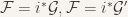 we also have
  via the diagonal embedding. Applying the extension lemma shows there is a coherent sheaf
  with
with  . Composing the inclusion
 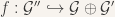 and the projection
  gives a morphism
  . By functorality we have
  . But
. But  , so
, so  is a morphism which induces the identity when restricted to .
Now we have an exact sequence

which gives us the relation ![[\text{coker}(g\circ f)] -[\mathcal{G}]+[\mathcal{G}''] -[\text{ker}(g\circ f)]=0](https://s0.wp.com/latex.php?latex=%5B%5Ctext%7Bcoker%7D%28g%5Ccirc+f%29%5D+-%5B%5Cmathcal%7BG%7D%5D%2B%5B%5Cmathcal%7BG%7D%27%27%5D+-%5B%5Ctext%7Bker%7D%28g%5Ccirc+f%29%5D%3D0&bg=f7f3ee&fg=333333&s=0&c=20201002) in . Since the restriction of to is the identity, the classes
in . Since the restriction of to is the identity, the classes ![[\text{coker}(g\circ f)],[\text{ker}(g\circ f)]](https://s0.wp.com/latex.php?latex=%5B%5Ctext%7Bcoker%7D%28g%5Ccirc+f%29%5D%2C%5B%5Ctext%7Bker%7D%28g%5Ccirc+f%29%5D&bg=f7f3ee&fg=333333&s=0&c=20201002) are represented by sheaves supported on ; thus these classes are trivial modulo the image of
are represented by sheaves supported on ; thus these classes are trivial modulo the image of  , and the relation obtained above becomes
 ![[\mathcal{G}'']=[\mathcal{G}]](https://s0.wp.com/latex.php?latex=%5B%5Cmathcal%7BG%7D%27%27%5D%3D%5B%5Cmathcal%7BG%7D%5D&bg=f7f3ee&fg=333333&s=0&c=20201002) . Repeating the argument for
. Repeating the argument for  instead of shows
 ![[\mathcal{G}'']=[\mathcal{G}']](https://s0.wp.com/latex.php?latex=%5B%5Cmathcal%7BG%7D%27%27%5D%3D%5B%5Cmathcal%7BG%7D%27%5D&bg=f7f3ee&fg=333333&s=0&c=20201002) hence the map is independent of choice of extension.
hence the map is independent of choice of extension.
To see the definition is well-defined on the quotient : we start with a short exact sequence of sheaves on

and find an extension of to . Since  , the extension lemma applies to give a coherent subsheaf with
  . From the exact sequence
  we get a commutative diagram with exact rows by applying and considering the natural cokernel exact sequence.

The left two vertical maps in the above are the identity, hence the right is an isomorphism. Thus, the coherent sheaf  extends
  since
since  . All together this completes the proof.
We’ll also need, similar to the Chow ring, a theorem on the homotopy invariance of G-theory. The proof is pretty long, and should probably be skipped (taken on faith) the first time seeing it.
(0.7) Proposition (homotopy): suppose  is a vector bundle of rank
  over with structure map
  . Suppose additionally
  have enough locally frees, and (hence also ) is reduced. Then the flat pullback
  is an isomorphism.
Proof. I’m not sure of a way to reduce the assumptions on . Let  be the 0-section. Then we have
  . By our assumption on this implies also the equality
  , hence
  is injective.
(To see  has finite Tor-dimesnion: the claim is local (we only need to check the stalks of Tor’s to see they vanish, since Tor commutes with limits) so we can assume is trivial; now observe the exact sequence
  on
on  (again this can be checked locally, so we can assume is affine, equal to
  , where the morphism comes from the map
 ![R[x_1,...,x_n]\rightarrow R[x_1,...,x_n]\rightarrow R](https://s0.wp.com/latex.php?latex=R%5Bx_1%2C...%2Cx_n%5D%5Crightarrow+R%5Bx_1%2C...%2Cx_n%5D%5Crightarrow+R&bg=f7f3ee&fg=333333&s=0&c=20201002) multiplying by all the variables then sending them all to 0); applying the exact functor
multiplying by all the variables then sending them all to 0); applying the exact functor  to the above exact sequence above gives a resolution of
 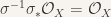 (equality since is a closed immersion) by sheaves for which the higher pullbacks will vanish in degree >2. That is to say, we needed to check the sheaves
 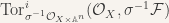 vanish outside a certain degree. To compute this sheaf we can take a resolution of either component by sheaves acyclic for the tensor product. We found a resolution of the left component with length 2. We then apply
 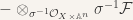 , and take the associated long exact sequence for Tor. All but the rightmost 4 terms vanish, proving that the 0 section has finite Tor dimension).
To see  is surjective we’ll reduce to the case of affine by using the localization sequence. Find an affine open subscheme
  which trivializes , with closed (reduced) complement
  . From the localization sequence we get the following commutative diagram with exact rows.

By a diagram chase, to prove the middle vertical arrow is surjective it suffices to prove the outer two are surjective. We can assume the leftmost is surjective by Noetherian induction ( is a variety so it’s Noetherian; if the left arrow isn’t surjective then repeat this argument with  . If the left arrow in that argument isn’t surjective repeat with a smaller closed subset. From this we get a decreasing chain of closed subsets, which eventually stabilizes (at a point in the worst case scenario — either way it will be affine). The argument we will give for will then apply and our inductive assumption shows the leftmost arrow in the above diagram is surjective.
Since the projection  factors
  , to show surjectivity of
  it suffices to show it for rank
  bundles. Here is where we will use the assumption is reduced. For any regular element (any element not a zero divisor) of
  , the localization sequence gives us the following commuting diagram with exact rows.
![\begin{matrix} G_0(\text{Spec}(R/f)) & \rightarrow & G_0(U=\text{Spec}(R)) & \rightarrow & G_0(R_f) & \rightarrow & 0\\ \downarrow & & \downarrow & & \downarrow & \\ G_0(\text{Spec}(R/f[t])) & \rightarrow & G_0(\text{Spec}(R[t])) & \rightarrow & G_0(\text{Spec}(R_f[t])) & \rightarrow & 0 \end{matrix}](https://s0.wp.com/latex.php?latex=%5Cbegin%7Bmatrix%7D+G_0%28%5Ctext%7BSpec%7D%28R%2Ff%29%29+%26+%5Crightarrow+%26+G_0%28U%3D%5Ctext%7BSpec%7D%28R%29%29+%26+%5Crightarrow+%26+G_0%28R_f%29+%26+%5Crightarrow+%26+0%5C%5C+%5Cdownarrow+%26+%26+%5Cdownarrow+%26+%26+%5Cdownarrow+%26+%5C%5C+G_0%28%5Ctext%7BSpec%7D%28R%2Ff%5Bt%5D%29%29+%26+%5Crightarrow+%26+G_0%28%5Ctext%7BSpec%7D%28R%5Bt%5D%29%29+%26+%5Crightarrow+%26+G_0%28%5Ctext%7BSpec%7D%28R_f%5Bt%5D%29%29+%26+%5Crightarrow+%26+0+%5Cend%7Bmatrix%7D&bg=f7f3ee&fg=333333&s=0&c=20201002)
We want to show the middle vertical arrow is a surjection. We’ll show this is true if is a field below. But, before we do that, we’ll show we can assume the leftmost vertical arrow in this diagram is surjective by Noetherian induction. The hardest part of this will be proving our induction step.
So, if is not a field, find a regular point  which is generated by a regular sequence
  . The localization sequence gives us the following commuting diagram with exact rows.
![\begin{matrix} G_0(\text{Spec}(R/(f_1,...,f_{n-1},g))) & \rightarrow & G_0(U=\text{Spec}(R/(f_1,...,f_{n-1}))) & \rightarrow & G_0((R/(f_1,...,f_{n-1}))_{g}) & \rightarrow & 0\\ \downarrow & & \downarrow & & \downarrow & \\ G_0(\text{Spec}(R/(f_1,...,f_{n-1},g)[t])) & \rightarrow & G_0(\text{Spec}(R/(f_1,...,f_{n-1})[t])) & \rightarrow & G_0(\text{Spec}((R/(f_1,...,f_{n-1}))_{g}[t]) & \rightarrow & 0 \end{matrix}](https://s0.wp.com/latex.php?latex=%5Cbegin%7Bmatrix%7D+G_0%28%5Ctext%7BSpec%7D%28R%2F%28f_1%2C...%2Cf_%7Bn-1%7D%2Cg%29%29%29+%26+%5Crightarrow+%26+G_0%28U%3D%5Ctext%7BSpec%7D%28R%2F%28f_1%2C...%2Cf_%7Bn-1%7D%29%29%29+%26+%5Crightarrow+%26+G_0%28%28R%2F%28f_1%2C...%2Cf_%7Bn-1%7D%29%29_%7Bg%7D%29+%26+%5Crightarrow+%26+0%5C%5C+%5Cdownarrow+%26+%26+%5Cdownarrow+%26+%26+%5Cdownarrow+%26+%5C%5C+G_0%28%5Ctext%7BSpec%7D%28R%2F%28f_1%2C...%2Cf_%7Bn-1%7D%2Cg%29%5Bt%5D%29%29+%26+%5Crightarrow+%26+G_0%28%5Ctext%7BSpec%7D%28R%2F%28f_1%2C...%2Cf_%7Bn-1%7D%29%5Bt%5D%29%29+%26+%5Crightarrow+%26+G_0%28%5Ctext%7BSpec%7D%28%28R%2F%28f_1%2C...%2Cf_%7Bn-1%7D%29%29_%7Bg%7D%5Bt%5D%29+%26+%5Crightarrow+%26+0+%5Cend%7Bmatrix%7D&bg=f7f3ee&fg=333333&s=0&c=20201002)
All such  which complete the regular sequence
  form a directed system where
  if
if  . From the surjectivity when our ring is a field, all of the maps on the left of these diagrams (indexed over regular elements ) are surjective. The right side of this diagram forms a directed system for total ring of fractions of
 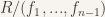 , which is a product of fields. What we’re left with is the following diagram
![\begin{matrix} \varinjlim_{g} G_0(\text{Spec}(R/(f_1,...,f_{n-1},g))) & \rightarrow & G_0(U=\text{Spec}(R/(f_1,...,f_{n-1}))) & \rightarrow & \bigoplus_i G_0(\text{Spec}(K_i)) & \rightarrow & 0\\ \downarrow & & \downarrow & & \downarrow & \\ \varinjlim_{g} G_0(\text{Spec}(R/(f_1,...,f_{n-1},g)[t])) & \rightarrow & G_0(\text{Spec}(R/(f_1,...,f_{n-1})[t])) & \rightarrow & \bigoplus_i G_0(\text{Spec}(K_i[t])) & \rightarrow & 0 \end{matrix}](https://s0.wp.com/latex.php?latex=%5Cbegin%7Bmatrix%7D+%5Cvarinjlim_%7Bg%7D+G_0%28%5Ctext%7BSpec%7D%28R%2F%28f_1%2C...%2Cf_%7Bn-1%7D%2Cg%29%29%29+%26+%5Crightarrow+%26+G_0%28U%3D%5Ctext%7BSpec%7D%28R%2F%28f_1%2C...%2Cf_%7Bn-1%7D%29%29%29+%26+%5Crightarrow+%26+%5Cbigoplus_i+G_0%28%5Ctext%7BSpec%7D%28K_i%29%29+%26+%5Crightarrow+%26+0%5C%5C+%5Cdownarrow+%26+%26+%5Cdownarrow+%26+%26+%5Cdownarrow+%26+%5C%5C+%5Cvarinjlim_%7Bg%7D+G_0%28%5Ctext%7BSpec%7D%28R%2F%28f_1%2C...%2Cf_%7Bn-1%7D%2Cg%29%5Bt%5D%29%29+%26+%5Crightarrow+%26+G_0%28%5Ctext%7BSpec%7D%28R%2F%28f_1%2C...%2Cf_%7Bn-1%7D%29%5Bt%5D%29%29+%26+%5Crightarrow+%26+%5Cbigoplus_i+G_0%28%5Ctext%7BSpec%7D%28K_i%5Bt%5D%29%29+%26+%5Crightarrow+%26+0+%5Cend%7Bmatrix%7D&bg=f7f3ee&fg=333333&s=0&c=20201002)
with leftmost arrow surjective since direct limits are exact, and rightmost arrow surjective from the result to be proved about fields. This proves the induction step necessary to assume the leftmost vertical arrow in our original sequence was surjective.
The same argument is now applied to reduce to the case of a field. By taking limits we reduce to the total ring of fractions of , which is a product of fields since is reduced.
Finally, the last thing to prove is the case was a field all along. In this case, ![R[t]](https://s0.wp.com/latex.php?latex=R%5Bt%5D&bg=f7f3ee&fg=333333&s=0&c=20201002) is a PID. All finitely generated modules over a PID are given by a free part isomorphic with
is a PID. All finitely generated modules over a PID are given by a free part isomorphic with ![R[t]^{\oplus n}](https://s0.wp.com/latex.php?latex=R%5Bt%5D%5E%7B%5Coplus+n%7D&bg=f7f3ee&fg=333333&s=0&c=20201002) and a torsion part isomorphic with a sum of pieces
and a torsion part isomorphic with a sum of pieces ![R[t]/(f)](https://s0.wp.com/latex.php?latex=R%5Bt%5D%2F%28f%29&bg=f7f3ee&fg=333333&s=0&c=20201002) . The exact sequence
. The exact sequence ![0\rightarrow R[t]\xrightarrow{\cdot f} R[t]\rightarrow R[t]/(f)\rightarrow 0](https://s0.wp.com/latex.php?latex=0%5Crightarrow+R%5Bt%5D%5Cxrightarrow%7B%5Ccdot+f%7D+R%5Bt%5D%5Crightarrow+R%5Bt%5D%2F%28f%29%5Crightarrow+0&bg=f7f3ee&fg=333333&s=0&c=20201002) shows the torsion summand is 0 in
shows the torsion summand is 0 in ![G_0(R[t])](https://s0.wp.com/latex.php?latex=G_0%28R%5Bt%5D%29&bg=f7f3ee&fg=333333&s=0&c=20201002) . Hence
. Hence ![G_0(R[t])\cong \mathbb{Z}](https://s0.wp.com/latex.php?latex=G_0%28R%5Bt%5D%29%5Ccong+%5Cmathbb%7BZ%7D&bg=f7f3ee&fg=333333&s=0&c=20201002) where the map takes a sheaf to its rank. Trivially
where the map takes a sheaf to its rank. Trivially  by the map taking a sheaf to is dimension as a vector space. Since the pullback map is given by
 ![[M]\mapsto [M\otimes_ R R[t]]](https://s0.wp.com/latex.php?latex=%5BM%5D%5Cmapsto+%5BM%5Cotimes_+R+R%5Bt%5D%5D&bg=f7f3ee&fg=333333&s=0&c=20201002) , the isomorphism
, the isomorphism ![G_0(R)\rightarrow G_0(R[t])](https://s0.wp.com/latex.php?latex=G_0%28R%29%5Crightarrow+G_0%28R%5Bt%5D%29&bg=f7f3ee&fg=333333&s=0&c=20201002) follows from the fact the dimension of a sheaf maps to the rank identically on .
follows from the fact the dimension of a sheaf maps to the rank identically on .
(0.8) Corollary: suppose  . Then
  .
.
As a suitable group for understanding the intersection theory of a variety , the G-theory of should depend on the subvarieties of in a crucial way. The next lemma says that this is the case; it also says that it may be more natural, when searching for generators of , to look at the geometry of .
(0.9) Proposition: the abelian group is generated by classes of coherent sheaves ![[\mathcal{O}_V]](https://s0.wp.com/latex.php?latex=%5B%5Cmathcal%7BO%7D_V%5D&bg=f7f3ee&fg=333333&s=0&c=20201002) as runs over the integral subvarieties of .
as runs over the integral subvarieties of .
Proof. To start, we reduce to the case is affine. To do this, we appeal to the localization sequence once again. Let  be the free abelian group on integral subvarieties of . We consider maps
  which take to .
Let be an open affine, and let  its reduced closed complement. Note the equalities
 ![j_*[\mathcal{O}_V]=[j_*\mathcal{O}_V]=[\mathcal{O}_{j(V)}]=[\mathcal{O}_V]](https://s0.wp.com/latex.php?latex=j_%2A%5B%5Cmathcal%7BO%7D_V%5D%3D%5Bj_%2A%5Cmathcal%7BO%7D_V%5D%3D%5B%5Cmathcal%7BO%7D_%7Bj%28V%29%7D%5D%3D%5B%5Cmathcal%7BO%7D_V%5D&bg=f7f3ee&fg=333333&s=0&c=20201002) and
and ![i^*[\mathcal{O}_X]=[i^*\mathcal{O}_X]=[\mathcal{O}_U]](https://s0.wp.com/latex.php?latex=i%5E%2A%5B%5Cmathcal%7BO%7D_X%5D%3D%5Bi%5E%2A%5Cmathcal%7BO%7D_X%5D%3D%5B%5Cmathcal%7BO%7D_U%5D&bg=f7f3ee&fg=333333&s=0&c=20201002) . Observe also the exact sequence
. Observe also the exact sequence  which is defined by inclusion and restriction (that the left is exact is trivial, that the right is exact follows from the existence of a closure, the middle is exact trivially — it even splits). Together we have shown the existence of the commutative diagram following.
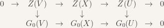
We want to show the middle vertical arrow is surjective. By assumption, to be shown below, the rightmost vertical arrow is surjective. If the leftmost arrow were surjective, we’d be done by a diagram chase. To see that we can assume the leftmost arrow is surjective, note that if it isn’t, we could repeat the above argument using ,  ,
,  for some
  . Continuing in this way, we get a chain of subvarieties
  , which eventually terminates at a closed point, call it
  . Since a closed point is affine, the leftmost vertical arrow is surjective, which shows
  is surjective by a diagram chase, which shows
  is surjective by a diagram chase, and so on.
To see the map is surjective for affine we recall the fact every finitely generated module  on an affine variety
  admits a filtration

with 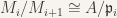 for some prime ideal
  . Adding over all integers the relations
 ![[M_{i+1}]-[M_i]+[A/{\mathfrak{p}_i}]](https://s0.wp.com/latex.php?latex=%5BM_%7Bi%2B1%7D%5D-%5BM_i%5D%2B%5BA%2F%7B%5Cmathfrak%7Bp%7D_i%7D%5D&bg=f7f3ee&fg=333333&s=0&c=20201002) obtained from short exact sequences
obtained from short exact sequences  gives a telescoping sum which ends with
 ![[M]=\sum_i[A/\mathfrak{p}_i]](https://s0.wp.com/latex.php?latex=%5BM%5D%3D%5Csum_i%5BA%2F%5Cmathfrak%7Bp%7D_i%5D&bg=f7f3ee&fg=333333&s=0&c=20201002) which completes the proof.
which completes the proof.
Proposition (0.11) below will be our main tool for computing the underlying abelian group for the varieties listed in the title. This proposition also refines the previous proposition, (0.9), in the special cases of the varieties in the title. In these cases, the varieties can be written as a disjoint union of locally closed subvarieties, called Schubert cells, each of which are isomorphic to an affine space of specific dimension. There is a partial ordering on these Schubert cells, induced from the Bruhat order of the Weyl group of the algebraic group acting on the given space. The closure of a Schubert cell, called a Schubert variety, is the union of the Schubert cells which are less or equal the given one in the Bruhat order. In particular, a Schubert variety is a union of smaller dimensional Schubert cells. This suggests we make the following
(0.10) Definition: suppose can be written as the finite disjoint union of irreducible locally closed subvarieties  with
with  , called cells, which satisfy the following two properties:
i) each cell is isomorphic to an affine space, 
ii) the closure of a cell is the union of other cells  .
.
Then we say has an affine stratification by the cells .
(0.11) Proposition: if admits an affine stratification, then is generated by the equivalence classes of the closures of the cells of the stratification, ![[X_i]](https://s0.wp.com/latex.php?latex=%5BX_i%5D&bg=f7f3ee&fg=333333&s=0&c=20201002) .
.
Proof. The proof is by induction on the number of cells. It can be found in the other post on the Chow ring as proposition (0.7). The only two properties needed in the proof are the localization exact sequence, proposition (0.6) in this post, and the homotopy property, proposition (0.7) in this post. So there really are no changes after replacing everywhere  by .
by .
We end this section with a special relation between the K-theory of a smooth variety , and the G-theory of . This is sometimes called the Cartan isomorphism, or Poincaré duality for K-theory. We’ll call it the Cartan isomorphism, since I’ve called K and G different theories.
(0.12) Proposition: if is a smooth variety, there are inverse isomorphisms

defined by ![\phi_{KG}([\mathcal{L}])=[\mathcal{L}]](https://s0.wp.com/latex.php?latex=%5Cphi_%7BKG%7D%28%5B%5Cmathcal%7BL%7D%5D%29%3D%5B%5Cmathcal%7BL%7D%5D&bg=f7f3ee&fg=333333&s=0&c=20201002) , and
, and ![\phi_{GK}([\mathcal{C}])= \sum_{i=1}^\infty(-1)^i[\mathcal{L}_i]](https://s0.wp.com/latex.php?latex=%5Cphi_%7BGK%7D%28%5B%5Cmathcal%7BC%7D%5D%29%3D+%5Csum_%7Bi%3D1%7D%5E%5Cinfty%28-1%29%5Ei%5B%5Cmathcal%7BL%7D_i%5D&bg=f7f3ee&fg=333333&s=0&c=20201002) where
where  is a resolution by finite locally free’s
  .
.
Proof. We have that  is surjective since every coherent sheaf on admits a finite resolution by finite locally frees (nonobvious result, it’s because is smooth and my varieties are separated). To see it’s injective, we show the inverse,
  is well-defined.
Define the map  from the free abelian group on coherent sheaves over to by the definition
 ![\mathcal{C}\mapsto \sum_{i=1}^\infty(-1)^i [\mathcal{L}_i]](https://s0.wp.com/latex.php?latex=%5Cmathcal%7BC%7D%5Cmapsto+%5Csum_%7Bi%3D1%7D%5E%5Cinfty%28-1%29%5Ei+%5B%5Cmathcal%7BL%7D_i%5D&bg=f7f3ee&fg=333333&s=0&c=20201002) for some finite resolution by finite locally frees . This is well-defined, i.e. it doesn’t depend on the choice of a resolution, because given two resolutions
for some finite resolution by finite locally frees . This is well-defined, i.e. it doesn’t depend on the choice of a resolution, because given two resolutions  , both quasi-isomorphic to
  , we have a map in the (bounded) derived category (of coherent sheaves) giving a distinguished triangle
  with
with  the cone of ; the cone is a complex which can be chosen to be a bounded complex of finite locally frees. The long exact cohomology sequence of this triangle (or a shift of this triangle) shows
 ![[c(f)]=0](https://s0.wp.com/latex.php?latex=%5Bc%28f%29%5D%3D0&bg=f7f3ee&fg=333333&s=0&c=20201002) and
and ![\sum_{i}(-1)^i[\mathcal{L}_{1,i}] -\sum_{j}(-1)^j[\mathcal{L}_{2,j}]=[c(f)]=0](https://s0.wp.com/latex.php?latex=%5Csum_%7Bi%7D%28-1%29%5Ei%5B%5Cmathcal%7BL%7D_%7B1%2Ci%7D%5D+-%5Csum_%7Bj%7D%28-1%29%5Ej%5B%5Cmathcal%7BL%7D_%7B2%2Cj%7D%5D%3D%5Bc%28f%29%5D%3D0&bg=f7f3ee&fg=333333&s=0&c=20201002) . Moving one of the sums to the other side shows is well-defined.
. Moving one of the sums to the other side shows is well-defined.
The map passes through the quotient , and we’ll call the induced map on the quotient . Hence it remains to show exists. We apply similar methods to the above to prove this claim: if we have a short exact sequence of coherent sheaves , then for two appropriate resolutions  , we get a distinguished triangle in the derived category
  . The long exact cohomology sequence of this triangle shows is a resolution of which can be chosen to be finite comprised of finite locally frees,
  . Then
![\phi_{GK}(\mathcal{G})=\sum_{i}(-1)^i[\mathcal{L}_{G,i}]](https://s0.wp.com/latex.php?latex=%5Cphi_%7BGK%7D%28%5Cmathcal%7BG%7D%29%3D%5Csum_%7Bi%7D%28-1%29%5Ei%5B%5Cmathcal%7BL%7D_%7BG%2Ci%7D%5D&bg=f7f3ee&fg=333333&s=0&c=20201002)
![=\sum_{i}(-1)^i [\mathcal{L}_{E,i}]-\sum_{i}(-1)^i [\mathcal{L}_{F,i}]=\phi_{GK}(\mathcal{E})-\phi_{GK}(\mathcal{F})](https://s0.wp.com/latex.php?latex=%3D%5Csum_%7Bi%7D%28-1%29%5Ei+%5B%5Cmathcal%7BL%7D_%7BE%2Ci%7D%5D-%5Csum_%7Bi%7D%28-1%29%5Ei+%5B%5Cmathcal%7BL%7D_%7BF%2Ci%7D%5D%3D%5Cphi_%7BGK%7D%28%5Cmathcal%7BE%7D%29-%5Cphi_%7BGK%7D%28%5Cmathcal%7BF%7D%29&bg=f7f3ee&fg=333333&s=0&c=20201002) .
.
Remark: The derived category is a red herring. One could write the proof only using the cone construction and the shift.
The Cartan isomorphism has a very interesting non-interesting application. The non-interesting aspect of the Cartan isomorphism is that it can be used to define a commutative, associative multiplication on the group whenever is a smooth variety. That is, we define a map  to be the composition
 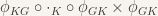 . I’ve added the subscripts
  here to keep track of the group the multiplication is defined on but, it will be dropped below.
The interesting part of this non-interesting application is that it gives a ring structure to the group which could appropriately be called an intersection product. We formalize this, and summarize the above discussion, in the following proposition.
(0.13) Proposition: given a smooth variety , there is an associative, commutative, bilinear multiplication on defined by

![([\mathcal{E}],[\mathcal{F}])\mapsto \sum_{i=0}^\infty (-1)^i [\text{Tor}_{\mathcal{O}_X}^i(\mathcal{E},\mathcal{F})]](https://s0.wp.com/latex.php?latex=%28%5B%5Cmathcal%7BE%7D%5D%2C%5B%5Cmathcal%7BF%7D%5D%29%5Cmapsto+%5Csum_%7Bi%3D0%7D%5E%5Cinfty+%28-1%29%5Ei+%5B%5Ctext%7BTor%7D_%7B%5Cmathcal%7BO%7D_X%7D%5Ei%28%5Cmathcal%7BE%7D%2C%5Cmathcal%7BF%7D%29%5D&bg=f7f3ee&fg=333333&s=0&c=20201002)
which agrees with the map  . This multiplication is called the intersection product of since, if
  ,
,  for two integral subvarieties
  intersecting properly and generically transversely, we have
 ![[\mathcal{O}_V]\cdot_G[\mathcal{O}_W]=[\mathcal{O}_{V\cap W}]](https://s0.wp.com/latex.php?latex=%5B%5Cmathcal%7BO%7D_V%5D%5Ccdot_G%5B%5Cmathcal%7BO%7D_W%5D%3D%5B%5Cmathcal%7BO%7D_%7BV%5Ccap+W%7D%5D&bg=f7f3ee&fg=333333&s=0&c=20201002) . If is a morphism of nonsingular varieties, then
. If is a morphism of nonsingular varieties, then  is a morphism of rings with respect to the intersection products.
Proof. That  , as defined above, agrees with the map by first transfering to K-theory can be seen as follows. Let
 ![[\mathcal{F}],[\mathcal{E}]](https://s0.wp.com/latex.php?latex=%5B%5Cmathcal%7BF%7D%5D%2C%5B%5Cmathcal%7BE%7D%5D&bg=f7f3ee&fg=333333&s=0&c=20201002) be two classes in . Choose two appropriate resolutions
be two classes in . Choose two appropriate resolutions  ,
,  of sheaves representing these classes. Then we have the equalities
![[\mathcal{F}]\cdot_G[\mathcal{E}]= \phi_{KG}(\sum_{i} (-1)^i[\mathcal{L}_i] \cdot_K \sum_{j}(-1)^j[\mathcal{M}_j])](https://s0.wp.com/latex.php?latex=%5B%5Cmathcal%7BF%7D%5D%5Ccdot_G%5B%5Cmathcal%7BE%7D%5D%3D+%5Cphi_%7BKG%7D%28%5Csum_%7Bi%7D+%28-1%29%5Ei%5B%5Cmathcal%7BL%7D_i%5D+%5Ccdot_K+%5Csum_%7Bj%7D%28-1%29%5Ej%5B%5Cmathcal%7BM%7D_j%5D%29&bg=f7f3ee&fg=333333&s=0&c=20201002)
![= \sum_{i}\sum_{j}(-1)^{i+j} [\mathcal{L}_i\otimes \mathcal{M}_j]](https://s0.wp.com/latex.php?latex=%3D+%5Csum_%7Bi%7D%5Csum_%7Bj%7D%28-1%29%5E%7Bi%2Bj%7D+%5B%5Cmathcal%7BL%7D_i%5Cotimes+%5Cmathcal%7BM%7D_j%5D&bg=f7f3ee&fg=333333&s=0&c=20201002)
![= \sum_{j}(-1)^j[\mathcal{F}\otimes \mathcal{M}_j]](https://s0.wp.com/latex.php?latex=%3D+%5Csum_%7Bj%7D%28-1%29%5Ej%5B%5Cmathcal%7BF%7D%5Cotimes+%5Cmathcal%7BM%7D_j%5D&bg=f7f3ee&fg=333333&s=0&c=20201002)
![= \sum_{j}(-1)^j[\mathcal{H}^j(\mathcal{F}\otimes \mathcal{M}^\bullet]](https://s0.wp.com/latex.php?latex=%3D+%C2%A0%5Csum_%7Bj%7D%28-1%29%5Ej%5B%5Cmathcal%7BH%7D%5Ej%28%5Cmathcal%7BF%7D%5Cotimes+%5Cmathcal%7BM%7D%5E%5Cbullet%5D&bg=f7f3ee&fg=333333&s=0&c=20201002)
![=\sum_{j}(-1)^j[\text{Tor}^j_{\mathcal{O}_X}(\mathcal{F},\mathcal{E})]](https://s0.wp.com/latex.php?latex=%3D%5Csum_%7Bj%7D%28-1%29%5Ej%5B%5Ctext%7BTor%7D%5Ej_%7B%5Cmathcal%7BO%7D_X%7D%28%5Cmathcal%7BF%7D%2C%5Cmathcal%7BE%7D%29%5D&bg=f7f3ee&fg=333333&s=0&c=20201002)
proving the first claim of the proposition.
The second claim of the proposition follows from the proof of [Stacks, Tag0B1I].
The final claim of the proposition follows from the fact that  and the fact that pullback commutes with tensor product and Tor.
Projective Space
This example is going to be lengthy but, we’ll get a very detailed calculation of  and
and  .
.
We’ll start by observing both and are generated as a group by at most  elements. To see this we can apply (0.11) to a particular filtration of
  to get the statement for . Because of the Poincaré duality (0.12), the same result will hold for . The filtration we use is

where for any  with
with  we have
  (this can be seen by taking succesively the vanishing locus of some coordinate functions
  ).
).
As mentioned before, this also shows is generated by at most elements because of Poincaré duality. Now we’ll show these generators form a basis of as a free abelian group consisting in exactly elements by exhibiting two distinct bases which are dual to each other with respect to a certain pairing.
To construct the necessary pairing we take the composition of the multiplication map on , with the Poincaré map , and then the pushforward to a point

![([\mathcal{E}],[\mathcal{F}])\mapsto [\mathcal{E}\otimes_{\mathcal{O}_X}\mathcal{F}]\mapsto [\mathcal{E}\otimes_{\mathcal{O}_X}\mathcal{F}]\mapsto \chi(\mathbb{P}^n,\mathcal{E}\otimes \mathcal{F}).](https://s0.wp.com/latex.php?latex=%28%5B%5Cmathcal%7BE%7D%5D%2C%5B%5Cmathcal%7BF%7D%5D%29%5Cmapsto+%5B%5Cmathcal%7BE%7D%5Cotimes_%7B%5Cmathcal%7BO%7D_X%7D%5Cmathcal%7BF%7D%5D%5Cmapsto+%5B%5Cmathcal%7BE%7D%5Cotimes_%7B%5Cmathcal%7BO%7D_X%7D%5Cmathcal%7BF%7D%5D%5Cmapsto+%5Cchi%28%5Cmathbb%7BP%7D%5En%2C%5Cmathcal%7BE%7D%5Cotimes+%5Cmathcal%7BF%7D%29.&bg=f7f3ee&fg=333333&s=0&c=20201002)
In the first component, consider the set of elements ![\mathscr{B}_1:=\{[\mathcal{O}_{\mathbb{P}^n}],[\mathcal{O}_{\mathbb{P}^n}(1)],\ldots, [\mathcal{O}_{\mathbb{P}^n}(n)]\}](https://s0.wp.com/latex.php?latex=%5Cmathscr%7BB%7D_1%3A%3D%5C%7B%5B%5Cmathcal%7BO%7D_%7B%5Cmathbb%7BP%7D%5En%7D%5D%2C%5B%5Cmathcal%7BO%7D_%7B%5Cmathbb%7BP%7D%5En%7D%281%29%5D%2C%5Cldots%2C+%5B%5Cmathcal%7BO%7D_%7B%5Cmathbb%7BP%7D%5En%7D%28n%29%5D%5C%7D&bg=f7f3ee&fg=333333&s=0&c=20201002) and in the second component consider the set of elements
and in the second component consider the set of elements ![\mathscr{B}_2:=\{[\mathcal{O}_{\mathbb{P}^n}],[\mathcal{O}_{\mathbb{P}^n}(-1)],\ldots, [\mathcal{O}_{\mathbb{P}^n}(-n)]\}](https://s0.wp.com/latex.php?latex=%5Cmathscr%7BB%7D_2%3A%3D%5C%7B%5B%5Cmathcal%7BO%7D_%7B%5Cmathbb%7BP%7D%5En%7D%5D%2C%5B%5Cmathcal%7BO%7D_%7B%5Cmathbb%7BP%7D%5En%7D%28-1%29%5D%2C%5Cldots%2C+%5B%5Cmathcal%7BO%7D_%7B%5Cmathbb%7BP%7D%5En%7D%28-n%29%5D%5C%7D&bg=f7f3ee&fg=333333&s=0&c=20201002) . Pairing these elements we get a matrix
. Pairing these elements we get a matrix  , which is upper triangular with 1’s on the diagonal, representing a map
  . Since the matrix
  has linearly independent columns and rows, we find
  ,
,  generate free subgroups in of rank . Since is generated by at most elements, this shows is a free abelian group of rank .
To see why 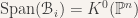 for
for  , choose a basis for . Then the inclusion
  is described by an integral matrix . The diagram
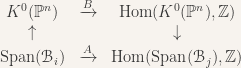
is commutative, with the matrix from the previous paragraph. Then the right vertical arrow is described by either or  depending if
  or
or  . Either way, this implies
  with
with  , hence
  . The previous discussion can be summarized:
(1.1) Proposition: There are presentations
![K^0(\mathbb{P}^n)=\mathbb{Z}\{[\mathcal{O}_{\mathbb{P}^n}],\ldots, [\mathcal{O}_{\mathbb{P}^n}(n)]\}](https://s0.wp.com/latex.php?latex=K%5E0%28%5Cmathbb%7BP%7D%5En%29%3D%5Cmathbb%7BZ%7D%5C%7B%5B%5Cmathcal%7BO%7D_%7B%5Cmathbb%7BP%7D%5En%7D%5D%2C%5Cldots%2C+%5B%5Cmathcal%7BO%7D_%7B%5Cmathbb%7BP%7D%5En%7D%28n%29%5D%5C%7D&bg=f7f3ee&fg=333333&s=0&c=20201002)
and
![K^0(\mathbb{P}^n)=\mathbb{Z}\{[\mathcal{O}_{\mathbb{P}^n}],\ldots, [\mathcal{O}_{\mathbb{P}^n}(-n)]\}](https://s0.wp.com/latex.php?latex=K%5E0%28%5Cmathbb%7BP%7D%5En%29%3D%5Cmathbb%7BZ%7D%5C%7B%5B%5Cmathcal%7BO%7D_%7B%5Cmathbb%7BP%7D%5En%7D%5D%2C%5Cldots%2C+%5B%5Cmathcal%7BO%7D_%7B%5Cmathbb%7BP%7D%5En%7D%28-n%29%5D%5C%7D&bg=f7f3ee&fg=333333&s=0&c=20201002)
which are dual to each other via the pairing described above.
(1.2) Corollary: We have a presentation
![G_0(\mathbb{P}^n)=\mathbb{Z}\{[\mathcal{O}_{\mathbb{P}^0}],[\mathcal{O}_{\mathbb{P}^1}],\ldots,[\mathcal{O}_{\mathbb{P}^n}]\}.](https://s0.wp.com/latex.php?latex=G_0%28%5Cmathbb%7BP%7D%5En%29%3D%5Cmathbb%7BZ%7D%5C%7B%5B%5Cmathcal%7BO%7D_%7B%5Cmathbb%7BP%7D%5E0%7D%5D%2C%5B%5Cmathcal%7BO%7D_%7B%5Cmathbb%7BP%7D%5E1%7D%5D%2C%5Cldots%2C%5B%5Cmathcal%7BO%7D_%7B%5Cmathbb%7BP%7D%5En%7D%5D%5C%7D.&bg=f7f3ee&fg=333333&s=0&c=20201002)
Proof. We now know that is a free abelian group generated by elements. We can refine our proof of (0.11) to obtain the above presentation as follows. We go by induction again and the localization exact sequence. Our base step is that  is freely generated by the class of its structure sheaf. For our induction hypothesis, assume for every
  we have
 ![G_0(\mathbb{P}^l)=\mathbb{Z}\{[\mathcal{O}_{\mathbb{P}^0}],...,[\mathcal{O}_{\mathbb{P}^l}]\}](https://s0.wp.com/latex.php?latex=G_0%28%5Cmathbb%7BP%7D%5El%29%3D%5Cmathbb%7BZ%7D%5C%7B%5B%5Cmathcal%7BO%7D_%7B%5Cmathbb%7BP%7D%5E0%7D%5D%2C...%2C%5B%5Cmathcal%7BO%7D_%7B%5Cmathbb%7BP%7D%5El%7D%5D%5C%7D&bg=f7f3ee&fg=333333&s=0&c=20201002) .
.
Now from the localization sequence there is a commutative diagram
![\begin{matrix} G_0(\mathbb{P}^{n-1}) & \xrightarrow{i_*} & G_0(\mathbb{P}^n) & \xrightarrow{j^*} & G_0(\mathbb{A}^n) & \rightarrow & 0 \\ \downarrow & & \downarrow & & \downarrow & &\\ \mathbb{Z}\{[\mathcal{O}_{\mathbb{P}^0}],...,[\mathcal{O}_{\mathbb{P}^{n-1}}]\} & \rightarrow & G_0(\mathbb{P}^n) & \rightarrow & \mathbb{Z}\{[\mathcal{O}_{\mathbb{A}^n}]\} & \rightarrow & 0 \end{matrix}](https://s0.wp.com/latex.php?latex=%5Cbegin%7Bmatrix%7D+G_0%28%5Cmathbb%7BP%7D%5E%7Bn-1%7D%29+%26+%5Cxrightarrow%7Bi_%2A%7D+%26+G_0%28%5Cmathbb%7BP%7D%5En%29+%26+%5Cxrightarrow%7Bj%5E%2A%7D+%26+G_0%28%5Cmathbb%7BA%7D%5En%29+%26+%5Crightarrow+%26+0+%5C%5C+%5Cdownarrow+%26+%26+%5Cdownarrow+%26+%26+%5Cdownarrow+%26+%26%5C%5C+%5Cmathbb%7BZ%7D%5C%7B%5B%5Cmathcal%7BO%7D_%7B%5Cmathbb%7BP%7D%5E0%7D%5D%2C...%2C%5B%5Cmathcal%7BO%7D_%7B%5Cmathbb%7BP%7D%5E%7Bn-1%7D%7D%5D%5C%7D+%26+%5Crightarrow+%26+G_0%28%5Cmathbb%7BP%7D%5En%29+%26+%5Crightarrow+%26+%5Cmathbb%7BZ%7D%5C%7B%5B%5Cmathcal%7BO%7D_%7B%5Cmathbb%7BA%7D%5En%7D%5D%5C%7D+%26+%5Crightarrow+%26+0+%5Cend%7Bmatrix%7D&bg=f7f3ee&fg=333333&s=0&c=20201002)
with  and
and  the respective inclusions and all vertical arrows isomorphisms. Since
 ![i_*([\mathcal{O}]_{\mathbb{P}^l})=[i_*\mathcal{O}_{\mathbb{P}^l}]=[\mathcal{O}_{\mathbb{P}^l}]](https://s0.wp.com/latex.php?latex=i_%2A%28%5B%5Cmathcal%7BO%7D%5D_%7B%5Cmathbb%7BP%7D%5El%7D%29%3D%5Bi_%2A%5Cmathcal%7BO%7D_%7B%5Cmathbb%7BP%7D%5El%7D%5D%3D%5B%5Cmathcal%7BO%7D_%7B%5Cmathbb%7BP%7D%5El%7D%5D&bg=f7f3ee&fg=333333&s=0&c=20201002) and
and ![j^*[\mathcal{O}_{\mathbb{P}^n}]=[\mathcal{O}_{\mathbb{A}^n}]](https://s0.wp.com/latex.php?latex=j%5E%2A%5B%5Cmathcal%7BO%7D_%7B%5Cmathbb%7BP%7D%5En%7D%5D%3D%5B%5Cmathcal%7BO%7D_%7B%5Cmathbb%7BA%7D%5En%7D%5D&bg=f7f3ee&fg=333333&s=0&c=20201002) we have is spanned by the elements
we have is spanned by the elements ![\{[\mathcal{O}_{\mathbb{P}^0}],...,[\mathcal{O}_{\mathbb{P}^n}]\}](https://s0.wp.com/latex.php?latex=%5C%7B%5B%5Cmathcal%7BO%7D_%7B%5Cmathbb%7BP%7D%5E0%7D%5D%2C...%2C%5B%5Cmathcal%7BO%7D_%7B%5Cmathbb%7BP%7D%5En%7D%5D%5C%7D&bg=f7f3ee&fg=333333&s=0&c=20201002) . That this is in fact a basis as a free group appears to be (to me at least) more subtle, but it follows from the fact any surjective endomorphism of free -modules is an isomorphism. To see this, extend the set
. That this is in fact a basis as a free group appears to be (to me at least) more subtle, but it follows from the fact any surjective endomorphism of free -modules is an isomorphism. To see this, extend the set ![\{[\mathcal{O}_{\mathbb{P}^0}],...,[\mathcal{O}_{\mathbb{P}^{n-1}}]\}](https://s0.wp.com/latex.php?latex=%5C%7B%5B%5Cmathcal%7BO%7D_%7B%5Cmathbb%7BP%7D%5E0%7D%5D%2C...%2C%5B%5Cmathcal%7BO%7D_%7B%5Cmathbb%7BP%7D%5E%7Bn-1%7D%7D%5D%5C%7D&bg=f7f3ee&fg=333333&s=0&c=20201002) to a basis
to a basis ![\{[\mathcal{O}_{\mathbb{P}^0}],...,[\mathcal{O}_{\mathbb{P}^{n-1}}], \alpha \}](https://s0.wp.com/latex.php?latex=%5C%7B%5B%5Cmathcal%7BO%7D_%7B%5Cmathbb%7BP%7D%5E0%7D%5D%2C...%2C%5B%5Cmathcal%7BO%7D_%7B%5Cmathbb%7BP%7D%5E%7Bn-1%7D%7D%5D%2C+%5Calpha+%5C%7D&bg=f7f3ee&fg=333333&s=0&c=20201002) and define the map
and define the map  by the identity on the first elements and sending
 ![[\mathcal{O}_{\mathbb{P}^{n}}]](https://s0.wp.com/latex.php?latex=%5B%5Cmathcal%7BO%7D_%7B%5Cmathbb%7BP%7D%5E%7Bn%7D%7D%5D&bg=f7f3ee&fg=333333&s=0&c=20201002) to
to  . This is surjective by assumption, so its also an isomorphism.
The ring structure on is clear. The ring structure on is less clear but, using (0.13) or using explicit locally free resolutions as in this post it can also be described fairly concretely.
We’ll conclude by computing the class of a hypersurface of degree  in as an element in . Since we know how to multiply
 ![[\mathcal{O}_{\mathbb{P}^{n-1}}]](https://s0.wp.com/latex.php?latex=%5B%5Cmathcal%7BO%7D_%7B%5Cmathbb%7BP%7D%5E%7Bn-1%7D%7D%5D&bg=f7f3ee&fg=333333&s=0&c=20201002) , this also computes the class of any subvariety which can be realized as consecutive proper and generically transverse intersections of hypersurfaces.
, this also computes the class of any subvariety which can be realized as consecutive proper and generically transverse intersections of hypersurfaces.
(1.3) Corollary: The class in of a degree hypersurface,  in , is given by
 ![[\mathcal{O}_S]=\sum_{i=1}^d (-1)^i {d\choose i} [\mathcal{O}_{\mathbb{P}^{n-i}}]](https://s0.wp.com/latex.php?latex=%5B%5Cmathcal%7BO%7D_S%5D%3D%5Csum_%7Bi%3D1%7D%5Ed+%28-1%29%5Ei+%7Bd%5Cchoose+i%7D+%5B%5Cmathcal%7BO%7D_%7B%5Cmathbb%7BP%7D%5E%7Bn-i%7D%7D%5D&bg=f7f3ee&fg=333333&s=0&c=20201002) .
.
Proof. This is just a Koszul complex; there is a 1-term resolution

where ![R=k[x_0,...,x_n]](https://s0.wp.com/latex.php?latex=R%3Dk%5Bx_0%2C...%2Cx_n%5D&bg=f7f3ee&fg=333333&s=0&c=20201002) . Taking the “tilde” operation to get the same thing for sheaves shows that in we find
. Taking the “tilde” operation to get the same thing for sheaves shows that in we find ![\phi_{GK}([\mathcal{O}_{S}])=[\mathcal{O}_{\mathbb{P}^n}]-[\mathcal{O}_{\mathbb{P}^n}(-d)]](https://s0.wp.com/latex.php?latex=%5Cphi_%7BGK%7D%28%5B%5Cmathcal%7BO%7D_%7BS%7D%5D%29%3D%5B%5Cmathcal%7BO%7D_%7B%5Cmathbb%7BP%7D%5En%7D%5D-%5B%5Cmathcal%7BO%7D_%7B%5Cmathbb%7BP%7D%5En%7D%28-d%29%5D&bg=f7f3ee&fg=333333&s=0&c=20201002) . Taking of this and applying the explicit description given in Computing locally free resolutions of a filtration of projective space completes the proof.
. Taking of this and applying the explicit description given in Computing locally free resolutions of a filtration of projective space completes the proof.
Interestingly, this is a key difference between and  for appropriate . The above proposition shows, even if we mod out by lower dimension subvarieties, that a sign must be taken account for in the sum. This isn’t at all true for .
References:
[Jav] Javanpeykar – The Grothendieck-Riemann-Roch Theorem with an application to covers of varieties. Can be found at the University of Leiden’s website.
[Lev] Levine – A short course in K-theory. Can be found on Marc Levine’s website.
[SGA6] Grothendieck, Berthelot, Illusie, et al. – Seminaire de geometrie algebrique du Bois Marie, Theorie des Intersections et Theoreme de Riemann-Roch. Can be found at the msri website.
[Stacks] The stacks project. Online resource for math

[…] post, and this one about K-theory, both serve the same purpose: to work out some explicit examples in intersection theory. The […]
LikeLike
[…] This turns out to be equivalent to computing the Koszul complex, and proving it’s a locally free resolution in the particular case of a polynomial ring with regular sequence . Here I’m thinking of as a field but any base ring will do. For a long time this was really confusing to me but, it turns out it really didn’t need to be. I’ll give an application at the very end of the post which relates the K-theory of projective space to the G-theory of projective space. This complements another blog of mine: Algebraic K-Theory revisited; the Grothendieck ring of Projective Space. […]
LikeLike
[…] I’ve rewritten the material in this post into a new blog post, Algebraic K-Theory revisited; the Grothendieck ring of Projective Space, with more detail. However, for a first encounter, the below is also […]
LikeLike
[…] Grothendieck Group of Algebraic Vector Bundles; Calculations of Affine and Projective Space; Algebraic K-Theory revisited; the Grothendieck ring of Projective Space; Split Semisimple Linear Algebraic Groups of Type […]
LikeLike
[…] (see [Quillen]), and the explicit calculation of the Grothendieck ring for projective space (see here). In particular, each individual Chow group is rank […]
LikeLike
[…] All of the K-theoretic background that is needed is contained in [EM1] but, not all of the information contained in that post will be used here; specifically, we just […]
LikeLike
[…] Algebraic K-Theory revisited; the Grothendieck ring of Projective Space […]
LikeLike