This post is going to be an amalgamation of some of the various ideas I’ve had in the last year, I guess. A year ago I thought about writing a post going over some of the representation theory of algebraic groups. This was a fools errand as the year in between taught me.
Instead, I’ve decided to write some posts that give details on the algebraic groups of type A — whatever that means at the moment if you haven’t heard it before. There are a couple of reasons why I want to do this: it’s good to work out some examples, I’ll have computations available for later, I eventually would like to have a pretty comprehensive list for algebraic groups of type ABCDEFG so why not start with A.
Since I’m repurposing an old blog, there might be a bit of heterogeneity in the content below. But I now realize that’s totally fine because this is a blog; it doesn’t have to be a treatise, or a textbook account, or have all the details.
Preliminaries
Let’s start out with some vocabulary. The objects I want to talk about are certain group schemes. These are objects which you should think of as being both a scheme, and a group. This is the analog in scheme theory of the concept of a Lie group in, say, complex manifold theory. There are problems with this interpretation from the get-go however. For example: how do you multiply a nonclosed generic point by a closed point, what does it mean to multiply two points of a scheme — given that the underlying set of a product is not the product of the underlying sets, and how does this form a group? This is, in my opinion, one of the biggest differences (or problems) one will first encounter when they try to generalize the idea of a Lie group to a scheme.
So how do we get around this problem? Well, we can generalize our definitions. What are the basic properties of a group? They are the existence of an identity, inverses, and the ability to multiply. Since we can’t use points directly, we’ll have to try to capture these properties with morphisms instead.
(1.1) Definition: A group scheme over a scheme  is a group object in the category of schemes over . This means a group scheme
  over is a scheme
  with morphisms
  ,
,  , and
, and  such that the following equalities hold:
a)  (associativity)
b)  (inverses)
c)  (identity); here
  is the canonical isomorphism
  provided by the fibered product.
The examples of group schemes this post will focus on are called split semisimple linear algebraic groups of type A. The type A part may be familiar from other areas of Lie theory — it comes from the root data we associate to our algebraic group. When I say algebraic group, I really just mean a group scheme over  , where is some field, and being over is shorthand for being over
  . But, to handle the simplest case first, we only want to deal with finite dimensional objects. This means we also impose a finite type (read as: finite dimensional) assumption when we speak about algebraic groups. Formally, we have just said:
(1.2) Definition: an algebraic group is a group scheme of finite type over a field .
Before I talk about why these definitions give us the ability to think of a scheme as a group, let me talk a little about its implications in the case is an affine algebraic group (when is a group scheme over an arbitrary scheme , the same conclusions could be made locally when is affine over . I won’t work in this generality. The most general situation I’ll consider is when is affine, and is affine over which, in particular, implies is affine).
Because of the equivalence between commutative rings and affine schemes, we get maps going in the other direction, satisfying the reverse conditions of definition 1.1, whenever we have an affine . The ring associated to an affine group scheme is then called a Hopf algebra.
(1.3) Definition: let  be a commutative ring. An Hopf algebra is an -algebra
  together with comultiplication, coinversion, and counit maps:
  ,
,  ,
,  which satisfy the relations
a)  (associativity)
b)  (inverses)
c)  (identity); here is the canonical isomorphism
  provided by the tensor product.
We’ll really only need to use Hopf algebras to show some properties of the underlying scheme of the algebraic group we are talking about. Possibly in another post (to be added), I’ll work out an example of how one can work with an algebraic group completely ring/scheme theoretically (but really only a simple one, probably  or
or  because I’ve done it before).
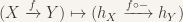
Now let’s return to why these properties in particular should capture the group theoretic properties an algebraic group is supposed to have. Often times it’s easier to work directly with the functor defined by the “points” of an algebraic group instead of the algebraic group itself. More generally, every scheme defines a functor  , and the group schemes can be identified as those schemes such that this functor factors
  with the last arrow being the forgetful functor (taking a group to its underlying set).
To see this, look again at the morphisms of definition 1.1. Try to convince yourself that, if these were given on a set instead of a scheme , then they would determine the structure of a group. Now observe, via the functor description of a scheme , the same arrows translate into natural transformations of functors

and so on… If we plug a scheme  into these functors, then these really are just maps of sets, and from here you’ve convinced yourself these maps determined a group structure (but now on the set
  ).
).
From this we can work more categorically. I’ll summarize the main points of what we will need in the below paragraphs but, if you want to see more detail then take a look at Alex Youcis’ blog here.
Choose a scheme . As I mentioned above, this defines a functor  . We can construct a category whose objects are functors from
  to
to  and whose morphisms are natural transformations of functors. Let’s call such a category
  and define a morphism of categories
  as the pair of maps
  ,
,  , and
, and  ,
,  . With this notation it’s possible to show
(1.4) Proposition: The morphism 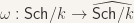 is a fully faithful embedding.
This is a great result for many reasons. Here are two that we’ll use fairly often. Proposition 1.4 says to give a morhpism of algebraic groups  it is equivalent to give a morphism of groups
  for every scheme . It’s actually incredibly easier to do the latter; it’s easier to check that we have defined a group homomorphism for every scheme than it is to check we have defined a morphism of schemes commuting with their group structures. The second use of prop. 1.4 is: say we define a functor
  and we can find a scheme such that
  for all schemes . Then it follows is the only scheme with this property. Said differently: schemes are uniquely determined by the functors they define. We’ll use both of these properties quite frequently.
But, before we continue, we can simplify this even further. One might wonder if we really need to check all schemes for these results to be true (maybe because general schemes are just affine schemes glued together). It turns out that we don’t. It’s sufficient to check these conditions on the affine schemes only. Formally,
(1.5) Lemma: Any functor  which factors through
  is uniquely determined by its restriction to
  .
.
Now, with a given scheme , I want to emphasize the scheme and not the functor  , so I’ll use (as is common practice) the notation
  . Other notational conventions I’ve chosen in this blog are as follows. An arbitrary field is denoted , and a finite type -algebra is denoted . I use
  for base change of
  along a morphism of affine schemes
  . I’ve already used this notation but, to avoid writing
  more than I want to, I’ll often identify and
  unless I use both simultaneously.
To conclude this section, we’ll end with some examples (some of which we’ll end up considering in the detail of the structure theory of algebraic groups in the following sections).
(1.6) Example: Define the functor  by
by  . We say it is represented by the scheme
  since, on affine schemes , we have
![h_{\mathbb{A}^1}(\text{Spec}(R))=\text{Hom}_{\mathsf{Sch}}(\text{Spec}(R),\mathbb{A}^1)=\text{Hom}_{\mathsf{Alg}}(k[X],R)=R:=\mathbb{G}_a(\text{Spec}(R)).](https://s0.wp.com/latex.php?latex=h_%7B%5Cmathbb%7BA%7D%5E1%7D%28%5Ctext%7BSpec%7D%28R%29%29%3D%5Ctext%7BHom%7D_%7B%5Cmathsf%7BSch%7D%7D%28%5Ctext%7BSpec%7D%28R%29%2C%5Cmathbb%7BA%7D%5E1%29%3D%5Ctext%7BHom%7D_%7B%5Cmathsf%7BAlg%7D%7D%28k%5BX%5D%2CR%29%3DR%3A%3D%5Cmathbb%7BG%7D_a%28%5Ctext%7BSpec%7D%28R%29%29.&bg=f7f3ee&fg=333333&s=0&c=20201002)
The only nontrivial equality in the above is a result of the universal mapping property of ![k[X]](https://s0.wp.com/latex.php?latex=k%5BX%5D&bg=f7f3ee&fg=333333&s=0&c=20201002) . This allows us to identify any morphism
. This allows us to identify any morphism ![k[X]\rightarrow R](https://s0.wp.com/latex.php?latex=k%5BX%5D%5Crightarrow+R&bg=f7f3ee&fg=333333&s=0&c=20201002) with the image of . We then give the set
with the image of . We then give the set ![\text{Hom}_{\mathsf{Alg}}(k[X],R)](https://s0.wp.com/latex.php?latex=%5Ctext%7BHom%7D_%7B%5Cmathsf%7BAlg%7D%7D%28k%5BX%5D%2CR%29&bg=f7f3ee&fg=333333&s=0&c=20201002) the group structure
the group structure  so that the functor factors through
  . This is called the additive group.
I used some formal terminology in the above, so I might as well include it as a definition.
(1.7) Definition: A functor  is represented by an object
  if
if  .
.
(1.8) Example: Define the functor  by
by  . A similar calculation to the above shows is represented by
  . Note for an affine scheme we find
  . This functor is called the vector group of dimension n. Most of the time I probably won’t write the subscript
  . Instead I’ll say
  of dimension , sticking with the convention from vector spaces.
(1.9) Example: For a vector space , the functor  is defined on affines by
  . When is finite dimensional then the choice of a basis for shows it is represented by the affine scheme
 ![A=\text{Spec}(k[X_{11},X_{12},...,X_{nn},1/\det])](https://s0.wp.com/latex.php?latex=A%3D%5Ctext%7BSpec%7D%28k%5BX_%7B11%7D%2CX_%7B12%7D%2C...%2CX_%7Bnn%7D%2C1%2F%5Cdet%5D%29&bg=f7f3ee&fg=333333&s=0&c=20201002) where
where  is the determinant of the
  matrix in the variables
  (e.g. for
  the determinant is
  ). If we’ve chosen a basis we’ll write
  instead of . To see this functor is represented by
  , we can proceed as in (Ex. 1.6.):
![h_A(\text{Spec}(R))=\text{Hom}_{\mathsf{Sch}}(\text{Spec}(R),A)=\text{Hom}_{\mathsf{Alg}}(k[X_{11},...,X_{nn}]_{\det},R)](https://s0.wp.com/latex.php?latex=h_A%28%5Ctext%7BSpec%7D%28R%29%29%3D%5Ctext%7BHom%7D_%7B%5Cmathsf%7BSch%7D%7D%28%5Ctext%7BSpec%7D%28R%29%2CA%29%3D%5Ctext%7BHom%7D_%7B%5Cmathsf%7BAlg%7D%7D%28k%5BX_%7B11%7D%2C...%2CX_%7Bnn%7D%5D_%7B%5Cdet%7D%2CR%29&bg=f7f3ee&fg=333333&s=0&c=20201002)
By the universal property of localization, ![\text{Hom}_{\mathsf{Alg}}(k[X_{11},...,X_{nn}]_{\det},R)](https://s0.wp.com/latex.php?latex=%5Ctext%7BHom%7D_%7B%5Cmathsf%7BAlg%7D%7D%28k%5BX_%7B11%7D%2C...%2CX_%7Bnn%7D%5D_%7B%5Cdet%7D%2CR%29&bg=f7f3ee&fg=333333&s=0&c=20201002) is the subset of
is the subset of ![\text{Hom}_{\mathsf{Alg}}(k[X_{11},...,X_{nn}],R)=R^{n^2}](https://s0.wp.com/latex.php?latex=%5Ctext%7BHom%7D_%7B%5Cmathsf%7BAlg%7D%7D%28k%5BX_%7B11%7D%2C...%2CX_%7Bnn%7D%5D%2CR%29%3DR%5E%7Bn%5E2%7D&bg=f7f3ee&fg=333333&s=0&c=20201002) such that
such that  is invertible. We give this set the group structure of matrix multiplication. This is the general linear group. The special case
  is written
  and called the multiplicative group.
Remark: In the above example,  is a group valued functor for any vector space . We can always describe a morphism to, or from, this functor. That is, we can always give morphisms between functors in the target category of (Prop 1.4.) but, we have only shown this will be a morphism of algebraic groups if is finite dimensional and the other functor in the morphism is represented by a scheme.
(1.10) Example: The special linear group is the quotient of at the ideal  . The group scheme structure is the same as in example (1.9). In particular, it is a sub-group scheme of .
Algebraic groups – type A
From here on out including any background is pretty much out of the question. I’m going to assume everything I know, and a couple of things I don’t know, about the structure theory of algebraic groups. All of our schemes are going to be over a fixed but arbitrary field and all of our group schemes are going to be affine (these are also called linear; I usually refer to them just as algebraic groups). The starting point for this series of blogs is going to be the following type of theorem.
(2.1) Theorem: split semisimple linear algebraic groups are classified, up to isomorphism, by the pair made of: the root system of and the fundamental group of .
The secondary starting point, and only for this post, is going to be the following lemma.
(2.2) Lemma:  is semisimple of type
  .
.
This will proved later in this post (above Theorem 2.8). But for now let’s take it on faith and study some of the geometric properties of  . There are multiple proofs for the following, and I’m not sure which proof is the cleanest. But here are some proofs which work, at least in the case of .
(2.3) Lemma: is smooth and connected.
Proof. Since is a variety (finite type over a field), it’s flat over its base. This means we only have to prove is geometrically regular to show that its smooth. Since we’ve already seen is an algebraic group (example 1.10), it’s sufficient to show is geometrically reduced. To do this it’s sufficient to show, after base changing to an algebraic closure of that the determinant minus 1 is irreducible. Hopefully you’re a sane person who picked the variables  to be outside any power of a transcendence base of the field over its prime field (which was really implicit in my definition of
  in the first place). The determinant has degree 1 in each of the variables
  so, if
  factors as
  for two polynomials
  then only one can have a
  term. Say
  does and write
  ,
,  . Similarly has degree 1 in
  , so one of has degree 1 in . It can’t be
  however, because then there would be a
  term in the determinant, which is visibly seen to be false by checking the determinant via cofactor expansion. A similar argument works with all the
  , so has all the terms. But again, this is all of them, as can be seen from expanding the determinant by the top row. We’re done then since
  implies is constant (as it can contain no variables else the left side has degree 2), and this in turn implies
  so that
  and is irreducible.
This also determines the dimension of as the dimension of minus 1. Since is an open subset of an irreducible variety, it has the same dimension as ![k[x_{11},...,x_{nn}]](https://s0.wp.com/latex.php?latex=k%5Bx_%7B11%7D%2C...%2Cx_%7Bnn%7D%5D&bg=f7f3ee&fg=333333&s=0&c=20201002) which is
which is  . We get, as a corollary,
(2.4) Corollary: has dimension  .
.
Proof. Given above.
Unfortunately that’s about as far as I can go in terms of the geometry of this algebraic group. It would be interesting if one could say more (computing the cohomology ring over  has been done, as an example, so we should be able to read off geometric information from there. For arbitrary fields I don’t know what one can say).
In a different direction, we could examine the algebraic structure of .
(2.5) Lemma: the diagonal subgroup variety is a split maximal torus. This can be realized as either 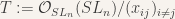 or as the subfunctor consisting of diagonal matrices.
Proof. We want to show that  is isomorphic with some power of . Using the functor approach this is pretty straightforward, just define an isomorphism
  by
by
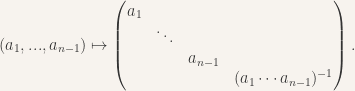
Hence this torus is split. To see that is maximal, we will show the centralizer of in is itself. To show this, we’ll use the fact that the Lie algebra of the centralizer is equal to the fixed points of the action of on the Lie algebra of . It will turn out that the Lie algebra of the centralizer has dimension  , which will complete the proof since the centralizer of a torus is smooth and connected so if we have
  this implies
  . The rest is proved in the following lemma.
(2.6) Lemma: the Lie algebra of is isomorphic with the -span of  and
and  where
where  and
and  run over the numbers from
  . The fixed points of the action of on
  are exactly the vectors .
Proof. The vector represents the matrix with 0’s every except the  th row and
  th column, where there is a 1 instead. Recall the Lie algebra of an algebraic group is defined to be the group-kernel of the map
 ![G(k[\varepsilon]/(\varepsilon^2))\rightarrow G(k)](https://s0.wp.com/latex.php?latex=G%28k%5B%5Cvarepsilon%5D%2F%28%5Cvarepsilon%5E2%29%29%5Crightarrow+G%28k%29&bg=f7f3ee&fg=333333&s=0&c=20201002) which is given by composing with the natural projection
which is given by composing with the natural projection ![\text{Spec}(k)\rightarrow \text{Spec}(k[\varepsilon]/(\varepsilon^2))](https://s0.wp.com/latex.php?latex=%5Ctext%7BSpec%7D%28k%29%5Crightarrow+%5Ctext%7BSpec%7D%28k%5B%5Cvarepsilon%5D%2F%28%5Cvarepsilon%5E2%29%29&bg=f7f3ee&fg=333333&s=0&c=20201002)
 . This is the tangent space at the identity of the group. To compute the Lie algebra of we first compute the Lie algebra for . These are all matrices with values in
 ![k[\varepsilon]/(\varepsilon^2)](https://s0.wp.com/latex.php?latex=k%5B%5Cvarepsilon%5D%2F%28%5Cvarepsilon%5E2%29&bg=f7f3ee&fg=333333&s=0&c=20201002) with invertible determinant and satisfying the condition if
with invertible determinant and satisfying the condition if  then
then  . All such matrices have to be equal to a sum
  where
where  is an arbitrary matrix of
  and all matrices of this form appear in the Lie algebra. Multiplying any two matrices of
  , say
, say  and
and  gives
gives

which allows us to define an isomorphism 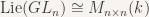 with the vector space of matrices with values in .
We identify with the sub-Lie algebra of consisting of those matrices with determinant 1. If , it’s easy to see the determinant of a matrix 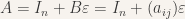 is equal
  . Computing the determinant of such a matrix via cofactor expansion (of the top row) we find
  with
with  the appropriate minors. All of summands vanish except the first, since can be computed by cofactor expansion along a column containing all terms degree 1 in
  . By induction this shows is an element of only when
  which happens if and only if
  . Under the isomorphism we’ve identified with those matrices having trace 0.
The claim about being spanned by the and where can then be seen as: this is a vector space of dimension , and is the kernel of the map  which is surjective. So they must be equal since they have the same dimension.
Finally, we come to the torus action. acts on via conjugation,  . We have inclusions
 ![G(R)\subset G(R[\varepsilon]/(\varepsilon^2))](https://s0.wp.com/latex.php?latex=G%28R%29%5Csubset+G%28R%5B%5Cvarepsilon%5D%2F%28%5Cvarepsilon%5E2%29%29&bg=f7f3ee&fg=333333&s=0&c=20201002) for every finite type -algebra and every algebraic group . We also have inclusions
for every finite type -algebra and every algebraic group . We also have inclusions ![G(k[\varepsilon]/(\varepsilon^2))\subset G(R[\varepsilon]/(\varepsilon^2))](https://s0.wp.com/latex.php?latex=G%28k%5B%5Cvarepsilon%5D%2F%28%5Cvarepsilon%5E2%29%29%5Csubset+G%28R%5B%5Cvarepsilon%5D%2F%28%5Cvarepsilon%5E2%29%29&bg=f7f3ee&fg=333333&s=0&c=20201002) . Evaluating the conjugation map on
. Evaluating the conjugation map on ![R[\varepsilon]/(\varepsilon^2)](https://s0.wp.com/latex.php?latex=R%5B%5Cvarepsilon%5D%2F%28%5Cvarepsilon%5E2%29&bg=f7f3ee&fg=333333&s=0&c=20201002) -points gives us then an action
-points gives us then an action ![T(R[\varepsilon]/(\varepsilon^2))\times SL_n(R[\varepsilon]/(\varepsilon^2))\rightarrow SL_n(R[\varepsilon]/(\varepsilon^2))](https://s0.wp.com/latex.php?latex=T%28R%5B%5Cvarepsilon%5D%2F%28%5Cvarepsilon%5E2%29%29%5Ctimes+SL_n%28R%5B%5Cvarepsilon%5D%2F%28%5Cvarepsilon%5E2%29%29%5Crightarrow+SL_n%28R%5B%5Cvarepsilon%5D%2F%28%5Cvarepsilon%5E2%29%29&bg=f7f3ee&fg=333333&s=0&c=20201002) . The inclusion
. The inclusion ![T(R)\subset T(R[\varepsilon]/(\varepsilon^2))](https://s0.wp.com/latex.php?latex=T%28R%29%5Csubset+T%28R%5B%5Cvarepsilon%5D%2F%28%5Cvarepsilon%5E2%29%29&bg=f7f3ee&fg=333333&s=0&c=20201002) and
and ![\text{Lie}(SL_n)\subset SL_n(k[\varepsilon]/(\varepsilon^2))\subset SL_n(R[\varepsilon]/(\varepsilon^2))](https://s0.wp.com/latex.php?latex=%5Ctext%7BLie%7D%28SL_n%29%5Csubset+SL_n%28k%5B%5Cvarepsilon%5D%2F%28%5Cvarepsilon%5E2%29%29%5Csubset+SL_n%28R%5B%5Cvarepsilon%5D%2F%28%5Cvarepsilon%5E2%29%29&bg=f7f3ee&fg=333333&s=0&c=20201002) defines the action of on . In short, it’s just conjugation. If
defines the action of on . In short, it’s just conjugation. If  is a diagonal matrix, multiplying out
  shows the claim.
Our next goal is to use this torus to study the root system of (or ). We’ll start by determining the Weyl group for .
(2.7) Lemma: The Weyl group of is isomorphic with  .
.
Proof. We can do this in two ways. I want to do it in both ways because they give different information and both are useful. The first way is directly from the following definition: the Weyl group of an algebraic group with respect to a split maximal torus is defined as the group  . This is a constant group scheme so we can identify it with its rational points, or with its points over an algebraic closure so that we could work directly with a quotient of groups. I’ll just give explicit representatives for this group, and defer that this is enough data until after we look at the second method of proof. We work with the maximal torus described in lemma 2.5.
Let  be the permutation matrix which transposes the rows and . This isn’t an element in
  but, it is up to a sign change. Multiply one of the rows of by
  (the choice doesn’t matter; they are all equivalent modulo ). Let
  be the group of
  elements generated by these matrices as runs over the numbers . No two are equivalent matrices mod
  , by comparing the position of 0’s in the matrices. To see that these are all the necessary representatives of
  , we will compute this group another way.
Note that the character group  of the split maximal torus of is a free abelian group of rank . Under the isomorphism
  described above, this group is spanned by the elements
  where goes through under the relation
  . A base for this lattice is given by
  where
where ![i\in [1, n-1]](https://s0.wp.com/latex.php?latex=i%5Cin+%5B1%2C+n-1%5D&bg=f7f3ee&fg=333333&s=0&c=20201002) for instance. On the other hand, the cocharacter group
for instance. On the other hand, the cocharacter group  is spanned by the elements
  where
where  is the map
  with
with  in the th spot and 1’s elsewhere. This can be considered in the lattice spanned by
  subject to the relation the sum of the coefficients must equal 0. If we call
  the lattice spanned by modulo
  and
and  the sublattice of the lattice spanned by subject to the relation the sum of the coefficients is 0, then we have a natural duality between and
  . This duality is realized by the pairing
  . Eventually I’ll write that paragraph less miserably.
Anyways, now we want to look at the root and the weight lattice. The root lattice is the sublattice of  spanned by the roots. Going back to our calculation of the action of on , we find
  . Hence the root lattice is spanned by those characters
  . This has index in but I won’t check this at moment. Via the above pairing, the coroots are exactly the elements , which span
  . This also shows will be simply connected (once we have shown it is semisimple).
The final piece of this proof is to show the reflections  generate . Then, as this group is isomorphic with we will have shown the Weyl group is . We will have also found representatives of the group explicitly since we originally found distinct elements and this shows there can be at most .
Now observe acts as the transposition swapping  on the characters
  . These reflections generate a subgroup of , and it is known the transpositions generate the entire group. So we are done.
That was a lot of work for seemingly not very much reward. But we’re now ready to prove Theorem 2.2. Actually, we could have done the first part of 2.2 at any time but, the second part had to wait until we had the computation of the Weyl group completed. I decided to do them together for whatever arbitrary reason.
Proof of 2.2. That is semisimple follows from the Lie-Kolchin theorem. We change base to an algebraic closure, and then we can assume a solvable subgroup is given as a subgroup of upper-triangular matrices. Since the radical of is normal, it is closed under conjugation so it must also be a subgroup of the lower-triangular matrices. Hence it is diagonal. Let  be a matrix contained in the radical of . Then a computation with shows
  which is diagonal only when
  . Hence all the entries of are the same. Therefore the radical is contained in the scalar matrices, which for is the group
  . The only connected subgroup variety of this is the trivial group, which shows is semisimple. To see has root system of type , we should start by finding a base for the given root system. Relative to the Borel subgroup of upper-triangular matrices, the simple roots are the
  . Taking the inner product
  gives 0 if
  , and 2 when
  . This is known as the root system of type .
I’m going to end this section with some facts about the family of type that I don’t want to prove at the moment (or don’t know how to prove at the moment).
(2.8) Theorem: The algebraic group is the simply connected simple algebraic group of type . It has center . The simple adjoint algebraic group of type is  . Thus, the almost simple algebraic groups of type are the quotients of by subgroups
  for varying and divisors
  of .
of .
Homogeneous varieties – type A
This section is, truth be told, the ulterior motive of this whole post. Unfortunately, it’s a broad enough topic I don’t want to include all of the details. Instead, this section will focus on examples. Moreover, all of the examples I’ll work out will be split (as opposed to twisted — what this means is I will consider Grassmannians and Flag varieties instead of their twisted forms, e.g. Severi Brauer varieties will not be discussed).
(3.1) Definition: Let be a vector space over . Define the functor  on points as

This is called the Grassmannian of -planes in .
To be more explicit about the defining conditions of this functor, we note that  is a -module by its right action. Then
  is an element of this set if there is a projective -module
  so that
  . The restriction maps on the functor are those coming from changing the base.
Note that there is symmetry in the definition. In other words the natural transformation  given by sending a summand to its complement defines a bijection on points, hence is naturally an isomorphism. There is also the obligatory mention,
  .
.
(3.2) Theorem: The Grassmannian is represented by a scheme, which we also call the Grassmannian, and we also denote by .
Reference. Here’s a reference.
The proofs in the Stacks project are more general than are being considered here. I’ve translated some of the conditions to the case where the base is a field.
(3.3) Definition: Let be a vector space over . Given a strictly increasing sequence of positive integers  we define the functor
  on points by

It’s called the  –split partial flag variety of type A.
(3.4) Theorem: For any sequence as above, the functor is represented by a scheme. We give this scheme the same name and notation as the functor it defines.
Proof Sketch. Choose a basis  for
for  . Then two flags in
  are given with respect to this basis, without loss of generality, by
  and
and  where the
  are sums in
  forming a sequence of linearly independent vectors.
  acts on the first flag, taking
  . By scaling we can assume the matrix this defines has determinant 1, and is hence in
  . Picking a point of
  for this action realizes the flag variety as a quotient of by the isotropy group of this point.
This is a sketch — not a proof. Mainly because one would need to check that the flag variety functor is the quotient of . This might mean adjusting the definition to include extensions by faithfully flat algebras… It’s actually a lot of work, and I don’t really know how to formalize it properly at the moment. That’s why I insist the above is only a sketch. The change won’t really affect us, whichever one it is.
Remark: Grassmannians are special cases of partial flag varieties.
(3.5) Example: Let’s compute the variety for  as the quotient
  by some parabolic subgroup
  (I know it’s parabolic because Grassmannians are projective — this follows from the Plücker embedding which I won’t go into detail about). Let be the standard basis vector for
  with 1 in the th position and 0’s elsewhere. A plane in is given by the (span of the) pair
  and we know the action of
  on the Grassmannian
  is transitive. We’ll find then to be the isotropy group
  . A computation shows
The subgroup of generated by these matrices will then do the trick. To be formal we should actually say the algebraic group defined by the vanishing of the equations 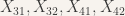 .
.
I want to continue this example by computing the Bruhat decomposition of (for purposes of a later post). The Plücker embedding actually shows embeds in  with one defining equation. In particular it has dimension 4. This is helpful as a guide but not strictly necessary. Let’s find a Levi decomposition for . That is, we’ll write
  where
where  is a reductive group and
  is a unipotent group.
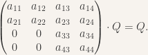
I claim  . In fact, I claim we have a decomposition, for every and every
  ,
,
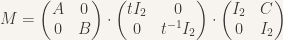
where  is the
  identity,
  are elements of
  ,
,  , and
, and  . To see this, write
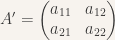 ,
, 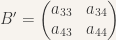 ,
, 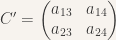 .
.
Observe,  since we can compute this using block matrices. Setting
  ,
,  ,
,  and
and  gives the desired decomposition.
From here it’s easy to see the Weyl group  , where is the same split torus we described in section 2. It’s
  corresponding to the subgroup of generated by the permutations
  and
and  . The Bruhat decomposition is given then by the recipe

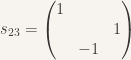
where the union takes place over one representative from each coset of  , and is the standard Borel of upper triangular matrices. Since the numerator has 24 elements, and the denominator has 4, we are consequently looking for 6 specific representatives. Here are some choices, one from each coset, in a list:
 ,
,  ,
,  ,
, 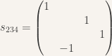 ,
,  ,
,  .
.
Counting inversions of the above permutations we can compute the Bruhat order for these elements. This means we find the length of each permutation to be  . From general theory, this calculates the dimensions of the given closures
 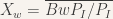 in
in  as
as 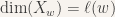 . To compute equations defining these invariants seems like too large a task at the moment, so I’ll stop here. This is enough for some purposes.
(3.6) Example: As a second example, we repeat the above computations for the flag variety  corresponding to the parabolic subgroup such that
  . Let represent the standard basis vectors, and consider the flag
  . Since
  acts transitively on , computing the isotropy group at
  will provide us with such a quotient.
But we can skip the calculation of the matrix group , if we want, because is the variety of complete flags. The stabilizer for the standard coordinate flag is just the Borel subgroup of upper triangular matrices, , which has been referred to throughout this whole blog. That is, is the subvariety of corresponding to the vanishing of the functions  .
.
To compute the Bruhat decomposition we can use the entire Weyl group  . More precisely, the decomposition appears in the form

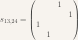
The six representatives are the six permutation matrices,
 ,
,  ,
,  ,
,  ,
, 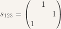 ,
, 
and the lengths of these elements are  .
.

[…] This post, and this one about K-theory, both serve the same purpose: to work out some explicit examples in intersection theory. The examples of Chow rings I’d like to compute are projective spaces, Grassmannians, and flag varieties. They are, depending on ones background, the simplest projective homogeneous varieties under the action of a split semisimple algebraic group of type A (that is to say, they are subvarieties of projective space that carry an action of an algebraic group, , where, on all -points, the action is also transitive). A current goal of mine is to be able to describe the intersection rings for various homogeneous varieties for every split semisimple algebraic group (all types – ABCDEFG); I can say with certainty this will not be achieved in the near future. Here however, it is achieved, for some homogeneous varieties under the action of a split semisimple algebraic group of type A. To get a good understanding of the below, knowing anything about algebraic groups is strictly unnecessary but, interested readers could find more information here. […]
LikeLike
Hey there 🙂 One nice thing you can read off about the algebraic geometry of of from its simply connectedness is the fact that it has trivial Picard group! This is kind of surprising to me–it’s not at all obvious why
 ![k[x_{ij}]/(\det-1)](https://s0.wp.com/latex.php?latex=k%5Bx_%7Bij%7D%5D%2F%28%5Cdet-1%29&bg=f7f3ee&fg=333333&s=0&c=20201002) is a UFD. But, as I’m sure you’re aware, for any semisimple group one has that
is a UFD. But, as I’m sure you’re aware, for any semisimple group one has that  is finite. If it were non-trivial then one could produce, using the Kummer sequence, a non-trivial cohomology class in
  (let’s work over
  for the moment) which is impossible since, as you remarked, it’s simply connected. In fact, one can go further and actually say that if
  is a semisimple group and
  is its universal cover, with kernel
  , then
  is the
  -points of the Cartier dual of
  (as a finite flat group scheme).
Also, I always found the Plucker embedding a bit confusing and hard to remember. You can see that the Grassmanian is projective since it’s a homogenous variety (so quasi-projective) and it evidently satisfies the valuative criterion (you can just choose a stable flat of lattices for a DVR!).
Nice post by the way!
LikeLike
Hey! Thanks for reading. I hadn’t really thought about the implication that the coordinate ring was a UFD. It’s certainly interesting that the Picard group can be identified with the rational points of the dual of the fundamental group. I don’t think I know enough to speak with any conviction (on top of a little bit of exhaustion from waking up early to TA today) but, the difficulty for me would be in seeing this for fields of char. p>0. I was unaware that the definition of fundamental group I was using (the kernel of a central isogeny from a universal cover) coincided with the etale fundamental group (well, dual to each other — in char. 0). The best I could find for this was this paper by Brion, (http://citeseerx.ist.psu.edu/viewdoc/download?doi=10.1.1.221.297&rep=rep1&type=pdf). I think I’ll need to look at this because it seems really interesting.
On a related note, I was thinking of reading through Grothendieck’s “Torsion homologique et sections rationelles” where I think he shows the Chow ring of a semisimple algebraic group is finite. Maybe I will combine these two observations in the format of a blog at some point…
That’s funny because I always found the valuative criterion impossible to use. I like that the Plucker embedding gives you a way to find equations describing the Grassmannian in projective space (even though doing so is usually unmanageable). Is it actually intuitive to use the valuative criterion (should I invest in learning it better)?
LikeLike
I mean, I certainly think so. I generally like to think of things explicitly in terms of their functor of points, so usually criteria that allow me to exploit this perspective are desirable.
Also to be clear, it’s of course not true that if is characteristic
  then
then  can be identified with
  . More naturally it’s that
  is
is  –namely it classifies geometrically connected finite etale covers of
  .
.
LikeLike
I should mention that if you’re interested in moduli spaces, then almost definitionally your’e going to have to work with (a modification) of the valuative criterion!
LikeLike
[…] Background posts: The Grothendieck Group of Algebraic Vector Bundles; Calculations of Affine and Projective Space; Algebraic K-Theory revisited; the Grothendieck ring of Projective Space; Split Semisimple Linear Algebraic Groups of Type A_n […]
LikeLike