Our goal for this blog post is to describe, for a smooth projective complex curve  , the group
  . In this regard, it is a natural continuation of the last post I wrote which gives calculations of the Grothendieck group of
  for all
  . This blog mainly consists of two big proofs (which probably should be skipped unless you’re looking for the proofs specifically). After these two proofs, we conclude with some explicit examples describable by (arbitrarily chosen) polynomials.
1. Theorem: Let be a smooth, projective curve. Then 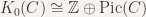 .
.
Proof. Our computation will rely on the Brown-Quillen spectral sequence of K-theory: for a regular scheme of finite type over a field, there is a convergent spectral sequence
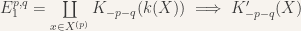
which satisfies 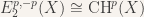 (here the notation
  means the set of points in codimension
  ; the filtration defined on the right hand side is the coniveau filtration, where the
  th step of the filtration is generated by sheaves with support in codimension
  ).
).
For a curve there are no codimension 2 points thus  and
and  . This gives isomorphisms
  ,
,  where, for a curve we have
  and for a smooth scheme we have
  . Using that
  (which is essentially definition) and
  (which is because our curve has only one irreducible component) we need only show there is an isomorphism
  .
.
This is manageable: we have a short exact sequence of abelian groups

with  . Since this map surjects onto
  , we need only choose a preimage of
  and it follows this sequence splits by sending a generator of to its preimage. This can also be summarized:
 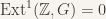 for every group
  .
.
We now specialize to the case where is defined over  , which allows us to give an explicit description of
  . We use analytic methods, which are described succinctly in [Algebraic Geometry – Hartshorne, Appendix B].
2. Proposition: For a smooth, projective, complex curve ,  where
where  is the genus of , and
  is a lattice in
  .
.
Proof. We will use the complex manifold  and obtain, using an application of Serre’s GAGA, results for the algebraic variety . Let
  be the constant sheaf
  ,
,  the sheaf of holomorphic functions
  , and
, and  the sheaf of invertible regular functions
  . There is then a short exact sequence of sheaves

with arrows  and
and  defined by
  and
and  respectively. This induces a long exact Čech cohomology sequence

Above we used the isomorphism  , an application of GAGA, along with the equivalence of Čech cohomology and the derived functor cohomology for coherent sheaves, and Grothendieck vanishing to conclude these groups are 0.
The data in  exactly classifies isomorphism classes of line bundles over , giving an isomorphism with
  . The equivalence of categories of line bundles given by GAGA gives an isomorphism
  .
.
Since any complex curve is locally contractible in the complex topology, we have isomorphisms  . If
. If  is the genus of , we can rewrite the above long exact sequence as

from which we also observe  is a surjection so that
  is an injection (hence a lattice). This implies there is a short exact sequence
  . Finally, since
  and the correspondence with elements of
  and extensions, we find
  as claimed. Of course, it is also possible here, as it was before, to define an explicit splitting of this sequence.
We’ll conclude by giving three examples of smooth projective curves with varying genus.
3. Example: Let ![C=\text{Proj}(\mathbb{C}[x,y,z]/(y^2z=x^3-xz^2))](https://s0.wp.com/latex.php?latex=C%3D%5Ctext%7BProj%7D%28%5Cmathbb%7BC%7D%5Bx%2Cy%2Cz%5D%2F%28y%5E2z%3Dx%5E3-xz%5E2%29%29&bg=f7f3ee&fg=333333&s=0&c=20201002) , which is the curve
, which is the curve  . It is smooth since it has nowhere vanishing Jacobian matrix, and it has genus
  by the degree-genus formula. Then for some nonzero
  we have
  and
and  .
.
Remark: I’m sure with more work one can find an explicit  for this isomorphism. Partly because, the curve provided is a complex elliptic curve – these curves are in bijection with quotients of the complex line by lattices
  – and the map described above embedding the torus
  into the Picard group is actually a well known map which, I think, identifies as the Jacobian variety of the elliptic curve. If you want to look up more, some keywords are: Jacobian variety, Albanese variety, Abel-Jacobi theorem.
Remark 2: Using resultants, one can show a polynomial of the form  is smooth if and only if
  . One can then check, as I just did, the Jacobian matrix for the polynomial
  doesn’t vanish whenever it is defined over a field of characteristic not
  .
.
4. Example: Let ![C=\text{Proj}(\mathbb{C}[x,y,z]/(x^5+y^5-z^5)](https://s0.wp.com/latex.php?latex=C%3D%5Ctext%7BProj%7D%28%5Cmathbb%7BC%7D%5Bx%2Cy%2Cz%5D%2F%28x%5E5%2By%5E5-z%5E5%29&bg=f7f3ee&fg=333333&s=0&c=20201002) . The curve is irreducible, which can be seen here using the Eisenstein criterion (we make one adjustment: if
. The curve is irreducible, which can be seen here using the Eisenstein criterion (we make one adjustment: if  then at
  we find one of
  to be a unit, hence one of is the monomial
  which is absurd). Using the Jacobian criterion, it follows this is a smooth curve. The degree-genus formula shows it is a genus 6 curve. Our principal result then says
  .
.
5. Example: Let ![C=\text{Proj}(\mathbb{C}[x,y,z]/(yz+x^2-2xz+z^2))](https://s0.wp.com/latex.php?latex=C%3D%5Ctext%7BProj%7D%28%5Cmathbb%7BC%7D%5Bx%2Cy%2Cz%5D%2F%28yz%2Bx%5E2-2xz%2Bz%5E2%29%29&bg=f7f3ee&fg=333333&s=0&c=20201002) . The degree-genus formula tells us this is a degree 0 curve. It is irreducible by the criterion here (using
. The degree-genus formula tells us this is a degree 0 curve. It is irreducible by the criterion here (using  and then arguing by homogeneity as in example 4). Smootheness is checked by the nonvanishing of the Jacobian matrix
  . Theorem 1 implies
  .
.

(Insert compliment about nice post here) 🙂
A few remarks:
1) There is a typo starting with “Since any complex curve…” Presumably you wanted to say that .
.
2) Saying that is zero seems a bit overkill to say that a short exact sequence ending in a free-module splits. 😛
3) The way to explicitly find the for an elliptic curve
  is actually quite explicit. Firstly, it’s not actually well-defined, in fact. Namely, the upper half-plane is a (fine) moduli space, but not for elliptic curves but, in fact, for elliptic curves with a trivialization of their homology (this is in the analytic category). In families, i.e. for a relative elliptic curve
  (where
  is a complex analytic space), this means fixing an isomorphism of
  with the trivial local systems
  . Anyways, back to the question: if we fix a basis
  of
of  then the
  is the ratio of
  and
and  for any non-vanishing invariant form
  on
on  .
.
4) It’s true that any elliptic curve is equal to its own Jacobian. What this means rigorously is that there is a canonical isomorphism between and
and  (as functors)–this is what gives
  a group structure. The
  subscript is not really important in the case of fields, but becomes more important when you want to define this
  thing on general schemes. Intuitively,
  (or rather the fppf sheafification of
  ) is a huge disjoint union of abelian varieties, and the choice of a basepoint of
  chooses one of these abelian varieties, and identifies
  with it.
Also, the Albanese is the dual of the Jacobian. Here there is really not so much of a difference except in functoriality.
5) In example 4 you can sidestep a lot of work, I believe. Namely, any hypersurface is connected, and if its smooth (which you verified by the Jacobian condition) it’s automatically irreducible. Indeed, if it weren’t then two irreducible fibers would intersect at some point and you can check that the local ring at that point is not integral, but regular local rings are integral, and smooth things have regular local rings.
6) In example , you don’t really need the powerful theorem–every genus zero curve with a rational point (so every genus
  smooth curve over a separably closed field) is just
  !
!
7) I know very little about K-theory sadly, but I’m curious as to whether or not one can reduce to the affine case? Namely from what I understand the fact that is
is  for
for  a Dedekind domain essentially follows from the structure theorem for projective modules. Is there any hope of doing an analogous thing here?
LikeLike
(Insert thank you, once again — this is easily one of my first computations and it’s always nice to get feedback).
1) Aww man 😦 we could have a hypersurface made of two disjoint curves. If I picked coordinates
 ![\mathbb{P}^1\times\mathbb{P}^1=\text{Proj}(k[w,x,y,z]/(xy-wz))](https://s0.wp.com/latex.php?latex=%5Cmathbb%7BP%7D%5E1%5Ctimes%5Cmathbb%7BP%7D%5E1%3D%5Ctext%7BProj%7D%28k%5Bw%2Cx%2Cy%2Cz%5D%2F%28xy-wz%29%29&bg=f7f3ee&fg=333333&s=0&c=20201002) then I could take for example the hypersurface
then I could take for example the hypersurface  — I think this is what will work). Of course, you are correct since I was working in the plane: by Bezout’s theorem every curve meets every other curve in the plane — and here a hypersurface is just a union of curves.
 is an affine smooth curve, there is an isomorphism
  given by
 ![[\mathcal{E}]\mapsto (\text{rk}(\mathcal{E}),[\text{det}(\mathcal{E})])](https://s0.wp.com/latex.php?latex=%5B%5Cmathcal%7BE%7D%5D%5Cmapsto+%28%5Ctext%7Brk%7D%28%5Cmathcal%7BE%7D%29%2C%5B%5Ctext%7Bdet%7D%28%5Cmathcal%7BE%7D%29%5D%29&bg=f7f3ee&fg=333333&s=0&c=20201002) where
where  is a vector bundle on
  . That this is an isomorphism follows by the structure theory of projective modules on a Dedekind domain (Theorem 5.6 in http://www.math.leidenuniv.nl/~edix/tag_2009/michiel_3.pdf), as you observed.
 is smooth and projective, then one really does get an isomorphism with the Chow ring of
  like so: the ring
  is naturally isomorphic to the (similarly defined) ring
  (the difference for me is that K uses locally free sheaves and G uses coherent sheaves — I wrote about this also here https://eoinmackall.wordpress.com/2017/09/24/algebraic-k-theory-revisited-the-grothendieck-ring-of-projective-space/). The ring
  admits a filtration
  where each term in the filtration is generated by sheaves with support codimension
  . There’s a natural map on the associated graded ring, maybe more natural to define in the other direction, which takes the class of a subvariety
  to the class
 ![[\mathcal{O}_V]](https://s0.wp.com/latex.php?latex=%5B%5Cmathcal%7BO%7D_V%5D&bg=f7f3ee&fg=333333&s=0&c=20201002) . It turns out that this map is always an isomorphism in codimension 0 and 1 (this is a consequence of the Grothendieck Riemann Roch without denominators but it can also be checked directly by elementary arguments). So to be precise, Hartshorne’s argument really is just describing this isomorphism without saying that this is the isomorphism he’s describing.
. It turns out that this map is always an isomorphism in codimension 0 and 1 (this is a consequence of the Grothendieck Riemann Roch without denominators but it can also be checked directly by elementary arguments). So to be precise, Hartshorne’s argument really is just describing this isomorphism without saying that this is the isomorphism he’s describing. is projective,
  is a point, and
  is an open affine complement. You can say that
  . To see this: use
  instead, noting they are isomorphic here and apply the localization sequence
  . The left map is actually injective in this case because
  is proper (one can compose with the structure map
  and note that
  is the identity). But I don’t think this really addresses the question because
  in general. This fails even for projective space.
 on a projective
  a filtration by sheaves
  so that the quotients are supported in affine pieces. Then one knows what the quotients are by the structure theory of Dedekind domains. Maybe I’d just get the above isomorphism in 1) by doing this though.
2) It’s absolutely overkill. But I quite like Ext groups.
3) That’s really interesting! I think these are sometimes called period integrals? I know someone who talks about integrating over (linearly independent) curves on Riemann surfaces but I’ve never been able to do it.
4) Maybe something you’d be interested in (I haven’t read much on the Picard functor) is this paper (https://arxiv.org/abs/1602.07491) by Liedtke. It’s more geometric but it seems to involve a study of the Picard functor in a case you might be interested in.
5) Not quite! Hypersurfaces don’t necessarily need to be connected (for example, inside of
6) Haha, yeah that’s true. I only found this out later though I think.
7) Kind of. The idea is nearly the same. Maybe I can say more about this:
If
If
Now, I can make some observations but I can’t say anything really definite at the moment:
1) Let me assume
2) If one did want to show this fact by trying to reduce to the affine case, it might not be a bad idea to try to use devissage in some way. Maybe it’s possible to construct, for any coherent sheaf
Yeah I’m not really sure. But maybe that answered the question still?
LikeLike
Thanks for the nice reply!
For 4) I meant hypersurface in (with
(with  )–I don’t think I’ve ever actually heard someone say hypersurface (out of context?) in something besides
  –maybe I should have said ‘projective hypesurfaces’. It’s ok there in all cases for the reason you said. Namely, if you have a hypesurface
  in
in  one can factorizat
  into irreducibles, in which case
  will be the union of the
  which are irreducible. One can then see, by codimension considerations, that these must pairwise intersect, and thus their union is connected. So, the correct statement is “every smooth hypersurface in
  for
for  is automatically irreducible.”
For 7), that’s along the lines I was thinking, and also couldn’t fully make it work. I thought there was a chance I was missing something. So, I think you addressed the question insofar as “do you see something I’m missing”.
Thanks again!
LikeLike
I can address 7) now. It actually does follow from the affine case.
You get a commutative diagram with exact rows from the chern character and localization sequences
and since the left and right vertical arrows are isomorphisms, so is the middle. Here we use that the left square commutes because of the Grothendieck-Riemann-Roch.
I guess this can also be checked directly, using the definition of the maps:
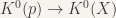 by
by ![[\mathcal{O}_p]\mapsto -[\mathcal{O}_X]+[\mathcal{O}(-p)]](https://s0.wp.com/latex.php?latex=%5B%5Cmathcal%7BO%7D_p%5D%5Cmapsto+-%5B%5Cmathcal%7BO%7D_X%5D%2B%5B%5Cmathcal%7BO%7D%28-p%29%5D&bg=f7f3ee&fg=333333&s=0&c=20201002)
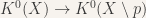 by
by ![[\mathcal{E}]\mapsto [\mathcal{E}|_{X\setminus p}\otimes \mathcal{O}_{X\setminus p}]](https://s0.wp.com/latex.php?latex=%5B%5Cmathcal%7BE%7D%5D%5Cmapsto+%5B%5Cmathcal%7BE%7D%7C_%7BX%5Csetminus+p%7D%5Cotimes+%5Cmathcal%7BO%7D_%7BX%5Csetminus+p%7D%5D&bg=f7f3ee&fg=333333&s=0&c=20201002)
 by
by ![[p]\mapsto [p]](https://s0.wp.com/latex.php?latex=%5Bp%5D%5Cmapsto+%5Bp%5D&bg=f7f3ee&fg=333333&s=0&c=20201002)
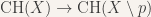 by
by ![[V]\mapsto [V\cap (X\setminus p)]](https://s0.wp.com/latex.php?latex=%5BV%5D%5Cmapsto+%5BV%5Ccap+%28X%5Csetminus+p%29%5D&bg=f7f3ee&fg=333333&s=0&c=20201002)
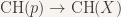
 by
by ![[\mathcal{O}_p]\mapsto [p]](https://s0.wp.com/latex.php?latex=%5B%5Cmathcal%7BO%7D_p%5D%5Cmapsto+%5Bp%5D&bg=f7f3ee&fg=333333&s=0&c=20201002)
 by
by ![[\mathcal{E}] \mapsto \text{rk}(\mathcal{E})+ c_1(\mathcal{E})](https://s0.wp.com/latex.php?latex=%5B%5Cmathcal%7BE%7D%5D+%5Cmapsto+%5Ctext%7Brk%7D%28%5Cmathcal%7BE%7D%29%2B+c_1%28%5Cmathcal%7BE%7D%29&bg=f7f3ee&fg=333333&s=0&c=20201002)
 by
by ![[\mathcal{E}]\mapsto \text{rk}(\mathcal{E})+ c_1(\mathcal{E})](https://s0.wp.com/latex.php?latex=%5B%5Cmathcal%7BE%7D%5D%5Cmapsto+%5Ctext%7Brk%7D%28%5Cmathcal%7BE%7D%29%2B+c_1%28%5Cmathcal%7BE%7D%29&bg=f7f3ee&fg=333333&s=0&c=20201002) .
.
LikeLike